Lab 13 - Autonomous Collaborative Search Part II
Maintained by: mikerb@mit.edu  Get PDF
1 Overview and Objectives
2 Preliminaries
3 Problem Description
3.1 The Search Region
3.2 The Object Laydown
3.2.1 Example File Format
3.2.2 Generating Hazard Files
3.3 Metrics of Success
3.4 Mission and Vehicle Constraints
3.4.1 Time
3.4.2 Top Speed
3.4.3 Limits on Inter-Vehicle Communication
3.4.4 Sensing During Turns
3.4.5 Sensor Configuration Options and Configuration Frequency
3.5 Dynamic Changes to the Rules
4 Assignments
4.1 Assignment 1 (check off) - Discuss Your Strategy with the 2.680 Staff
4.2 Assignment 2 (check off) - Confirm Distributed Operation of Initial Mission
4.3 Assignment 3 - Prepare for the competition time window
4.4 Assignment 4 - Prepare a 5-10 Minute Brief of your Solution
5 Competition Parameters
6 Instructions for Handing In Assignments
6.1 Requested File Structure
6.2 Important Dates
1 Overview and Objectives
The focus of this week's lab is to continue work on the autonomous collaborative search challenge problem in preparation for in-class competition Thursday April 12th 2018. In the previous lab the initial focus was on obtaining and running the baseline mission, and augmenting it to allow vehicles to share information to produce a single collective report. In this lab the focus is to continue to improve your solution. You will need to consider:

- the probability/likelihood of an object being an actual hazard, rather than just a benign object. You'll need to consider the quality of the detection sensor and classification algorithm. You'll need to consider what can be inferred from multiple passes over the same object, with perhaps different sensor conclusions. You will also want to consider how to use the sensor information from your other vehicle.
- the relative penalties of missed detections and false alarms when deciding whether to include an object in the list of hazards in your final report. Your team's final certainty measurement about each object should be weighed with the relative penalties to give yourself the best chance for a high score. Remember that the penalty structure may change at competition time, as described in Section 3.5.
- adaptive path planning. You very likely will find it advantageous to adapt one or both of your vehicle's paths away from the basic lawnmower pattern to perhaps re-visit and re-collect sensor information about objects of initial interest, or objects that you determine are on the boundary of what otherwise would be a clear reporting decision.
A summary of today's topics:
- Continue the Autonomous Collaborative Search Challenge Problem
- Make use of the classification component of the Hazard Sensor
- Implement probability/certainty reasoning to your mission structure
- Implement risk/reward reasoning based on sensor certainty and competition metrics
- Implement path re-planning to improve your mission effectiveness
2 Preliminaries
Make Sure You Have the Latest Updates [top]
Always make sure you have the latest code:
  $ cd moos-ivp
  $ svn update
And rebuild if necessary:
  $ ./build-moos.sh
  $ ./build-ivp.sh
Make Sure Key Executables are Built and In Your Path [top]
This lab does assume that you have a working MOOS-IvP tree checked out and installed on your computer. To verify this make sure that the following executables are built and findable in your shell path:
  $ which MOOSDB
  /Users/you/moos-ivp/bin/MOOSDB
  $ which pHelmIvP
  /Users/you/moos-ivp/bin/pHelmIvP
If unsuccessful with the above, return to the steps in Lab 1:
http://oceanai.mit.edu/ivpman/labs/machine_setup?
Where to Build and Store Lab Missions [top]
As with previous labs, we will use your version of the moos-ivp-extend tree, which by now you should have re-named something like moos-ivp-janedoe, where your email may be janedoe@mit.edu. In this tree, there is a missions folder:
  $ cd moos-ivp-janedoe
  $ ls
  CMakeLists.txt  bin/       build.sh*    clean.sh*    docs/    missions/
  src/            README     build/       data/        lib/     scripts/
For each distinct assignment in this lab, there should be a corresponding subdirectory in a lab_13 sub-directory of the missions folder, typically with both a .moos and .bhv configuration file. See Section 6.1 for the full requested file structure.
Documentation Conventions [top]
To help distinguish between MOOS variables, MOOS configuration parameters, and behavior configuration parameters, we will use the following conventions:
- MOOS variables are rendered in green, such as IVPHELM_STATE, as well as postings to the MOOSDB, such as DEPLOY=true.
- MOOS configuration parameters are rendered in blue, such as AppTick=10 and verbose=true.
- Behavior parameters are rendered in brown, such as priority=100 and endflag=RETURN=true.
More MOOS / MOOS-IvP Resources [top]
- The slides from class on multi-vehicle autonomy:
http://oceanai.mit.edu/2.680/docs/2.680-10-multiple_vehicles_2018.pdf - The uFldMessageHandler documentation
http://oceanai.mit.edu/ivpman/apps/uFldMessageHandler - The uFldNodeComms documentation
http://oceanai.mit.edu/ivpman/apps/uFldNodeComms
- The slides from class on Collaborative Search:
http://oceanai.mit.edu/2.680/docs/2.680-13-collaborative_search_2018.pdf - The uFldHazardSensor documentation
http://oceanai.mit.edu/ivpman/apps/uFldHazardSensor - The uFldHazardMetric documentation
http://oceanai.mit.edu/ivpman/apps/uFldHazardMetric - The uFldHazardMgr documentation
http://oceanai.mit.edu/ivpman/apps/uFldHazardMgr
3 Problem Description
This section describes the problem parameters, mission constraints and format for a vehicle to generate a report at the end of a mission. The following five points are discussed:
- A search region
- An object lay-down
- Metrics of success
- Mission and vehicle constraints
- Reporting criteria
Values for the first four components are discussed below, but may be altered at competition time. The idea is to have a canonical problem to focus on for development, which will be part of the competition, and have a to-be-determined variation of the problem also part of the competition. The latter will help judge how general the individual submitted solution may be.
3.1 The Search Region [top]
The simulated hazard region will be within a polygon with the following four vertices:
- (-150, -75)
- (-150, -400)
- (400, -400)
- (400, -75)
The initial search region is chosen to be rectilinear to simplify a lawnmower pattern generation for a waypoint behavior. See the documentation for this behavior. A pattern may be given to the behavior simply by specifying the characteristics of the lawnmower pattern without having to explicitly determine all the points.
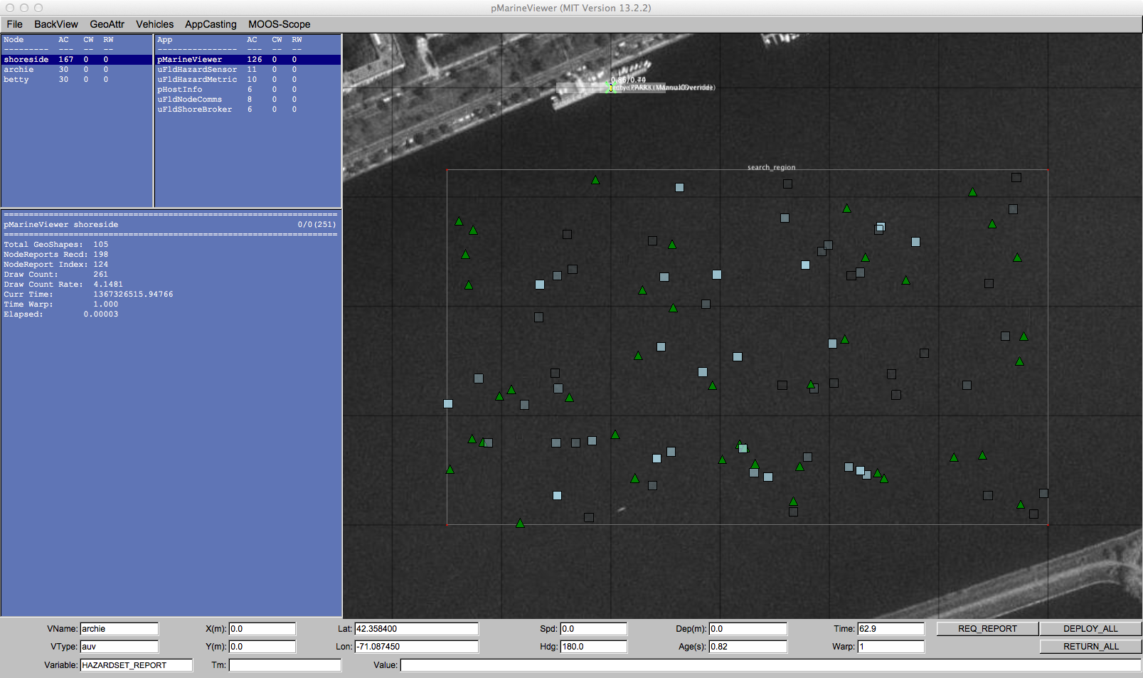
Figure 3.1: The search region is given in the local coordinates of the MIT Sailing Pavilion on the Charles River. The local (0,0) position is on the dock where vehicles are launched and recovered.
3.2 The Object Laydown [top]
The object laydown is defined in a hazard file, not known to the vehicle at run time. It contains a set of objects, some of which are of type hazard and some of type benign. Identifying and correctly determining the type of these objects is the goal of the mission. For simulation testing and development purposes, a number of hazard files are provided in the baseline mission. A simple example, used as the default in the baseline mission, is shown in Figure 3.1.
3.2.1 Example File Format [top]
A hazard file is simply a text file, with line for each object. An example is below. This is discussed in greater detail in the uFldHazardSensor documentation.
 hazard = x=165,y=-91,label=32,type=hazard
 hazard = x=21,y=-88,label=85,type=hazard
 hazard = x=370,y=-219,label=23,type=hazard
 hazard = x=-149,y=-318,label=92,type=hazard
 o o o
 hazard = x=189,y=-326,label=75,type=benign
 hazard = x=52,y=-164,label=8,type=benign
 hazard = x=174,y=-190,label=46,type=benign
 hazard = x=357,y=-177,label=40,type=benign
 hazard = x=211,y=-315,label=38,type=benign
3.2.2 Generating Hazard Files [top]
A hazard file may be generated with a provided command line tool, to allow the user to perform more extensive tests of their choosing. The gen_hazards utility is distributed with the moos-ivp code, and an example command line invocation is below. This tool is discussed in greater detail in the uFldHazardSensor documentation.
$ gen_hazards --polygon=-150,-75:-150,-400:400,-400:400,-75 --objects=5,hazard --objects=8,benign
3.3 Metrics of Success [top]
The scoring metrics are as follows:
- 150: Penalty for missed hazard
- 25: Penalty for false alarm
- 300: Penalty for being late (later than 7200 seconds)
- 0.25: Additionaly late penalty applied to each second of lateness.
3.4 Mission and Vehicle Constraints [top]
There are handful of mission and vehicle constraints enforced to keep everyone on the same playing field.
3.4.1 Time [top]
The maximum mission time is 7200 seconds, or 2.0 hours. This value was chosen, in part, since most computers can support a MOOS time warp of 10-20x realtime or much higher on newer systems. A time warp of 20 allows a full mission to be simulated in less than ten minutes. The mission time constraint has a variable penalty associated with it:
- 300: Penalty for being late (1 second later than 7200 seconds), and
- 0.25: Additional late penalty applied to each second of lateness.
3.4.2 Top Speed [top]
Vehicles will be limited to a speed of 2.0 meters per second. There is no penalty in terms of sensor performance or comms for moving at the top speed. Vehicles moving over the top speed will essentially automatically disable their own sensors until the speed is reduced.
3.4.3 Limits on Inter-Vehicle Communication [top]
Communications between vehicles will limited in range, frequency and bandwidth. This will need to be accounted for both during the mission for collaboration, and at the end of the mission for fusing the two vehicles' belief states into a single hazardset report. The restrictions will be
- Range: Communications limited to 100 meters
- Frequency: Communications will be limited to once per 60 seconds
- Bandwidth: Each message will be limited to 100 characters
These configurations are enforced in the uFldNodeComms configuration. This module is on the shoreside and will be configured by the competition organizers, and is configured with these values in the baseline mission. You will be running your own shoreside MOOS community during development, but you should not change this configuration in your uFldNodeComms configuration to ensure you are developing in an environment similar to the competition. Remember that a message that fails to be sent, due to one of the above criteria, will not be queued for later re-sending. You should handle the possibility that message may be dropped.
3.4.4 Sensing During Turns [top]
The simulated sensor will be rendered off during turns of 1.5 degrees per second. This is discussed in greater detail in the uFldHazardSensor documentation.
3.4.5 Sensor Configuration Options and Configuration Frequency [top]
Vehicles will be allowed to set their sensor configuration once at the outset. Attempts to switch configurations after the outset will simply be ignored. You may, however, switch the the  setting (and corresponding PFA setting) as often as you like.
Your sensor configuration options will be:
   sensor_config = width=5, exp=8, class=0.88, max=1
   sensor_config = width=10, exp=6, class=0.70
   sensor_config = width=25, exp=4, class=0.63
   sensor_config = width=50, exp=2, class=0.55
See the documentation for uFldHazardSensor on what this entails in terms of the ROC curve performance of the sensor, and how the vehicle may request a particular configuration. The first sensor setting, with width=5 may be enabled for at most one vehicle.
3.5 Dynamic Changes to the Rules [top]
As mentioned at the outset, baseline values are provided for the initial development and first phase of the competition for the following parameters:
- A search region
- An object lay-down
- Metrics of success
- Mission and vehicle constraints
Part of the competition will test exactly on the given baseline parameters. Part of the competition will test on parameters only known at competition time. How will those parameters be made available? They will be set on the shoreside in the uFldHazardMetric application and posted to the shoreside MOOSDB and shared out to the vehicles.
 UHZ_MISSION_PARAMS = "penalty_missed_hazard=150,penalty_false_alarm=25,max_time=600,
                       penalty_max_time_over=300,penalty_max_time_rate=0.5,
                       search_region=pts={-150,-75:-150,-400:400,-400:400,-75}"
If you run the baseline mission and scope the MOOSDB on one of the vehicles, you will notice that a publication similar to the above has been made, originating in the shoreside in the uFldHazardMetric application. For example, after launching the baseline mission, in a separate terminal window you should see something like:
  $ cd moos-ivp/ivp/missions/m10_jake
  $ uXMS targ_betty.moos UHZ_MISSION_PARAMS
  Mission File was provided: targ_betty.moos
  uXMS_630 thread spawned
  starting uXMS_630 thread
  ----------------------------------------------------
  |       This is an Asynchronous MOOS Client        |
  |       c. P. Newman U. Oxford 2001-2012           |
  ----------------------------------------------------

  o o o

  ===================================================================
  uXMS_630 betty                                               0/0(1)
  ===================================================================
  VarName             (S)ource          (T)  (C)ommunity  VarValue (SCOPING:EVENTS)
  ------------------  ----------------  ---  ----------  -------------------------
  UHZ_MISSION_PARAMS  uFldHaz..dMetric       shoreside   "penalty_missed_hazard=150,
  penalty_false_alarm=25,max_time=600,penalty_max_time_over=300,penalty_max_time_rate=0.5,
  search_region=pts={-150,-75:-150,-400:400,-400:400,-75}"
Presently, in the baseline mission, this information is not being handled by either vehicle. If the mission were to change, the vehicle would not adjust. But this is why it is a baseline mission; it's not complete and is meant to be a competition starting point.
In this competition, the only parameters that will change are the penalty values, the threat lay-down, and the mission time. The top vehicle speed and sensor properties will not be changed. You can assume the values used in the baseline mission.
4 Assignments
The primary assignment for this lab is to participate in the in-class competition next Thursday April 12th, 2018. Below are a few things that should be checked along the way to keep things on-track.
4.1 Assignment 1 (check off) - Discuss Your Strategy with the 2.680 Staff [top]
By the end of the first day of the lab, you should plan to have a strategy discussion with one of the TAs regarding you approach to (a) representing liklihood results (b) sharing liklihood results between vehicles, (c) adaptive path planning, (d) inter-vehicle communications and anything else you are considering in your overall implementation.
There is no right solution to this problem, and the results-oriented nature of a competition with metrics is indeed intended to allow a diverse set of possible approaches. But we feel it is generally very useful to approach the problem with a clear general initial stategy. We want to encourage and verify that you do this, and give you a chance to sanity check your approach to a non-competitor.
4.2 Assignment 2 (check off) - Confirm Distributed Operation of Initial Mission [top]
The single most important component to your lab grade is that something works when it comes to the in-class competition. Here are two traps to avoid:
- Don't fall into the trap of designing a super clever implementation that doesn't work at all on the competition date, due to perhaps some minor bug. We encourage you to start with and maintain a simpler version of your mission as a fall-back. This can be something pretty close to the baseline solution if you choose.
- Don't fall into the trap of not being able to run in a distributed manner on the test-date. The competition will have a single shoreside display set up by the instructor, and each student will simulate one vehicle on their laptop.
By the end of Tuesday's lab (April 10th, 2018), you should be able to demonstrate that your two machines are able to connect and run some simple version of your mission connected to the instructor machine running a shoreside mission.
4.3 Assignment 3 - Prepare for the competition time window [top]
We will be holding the competition on Thursday April 12th, from 930-1230, in Beaver Works, our normal classroom. Prior to the competition, please determine the highest timewarp your computers will tolerate for the mission. It makes a difference in gauging the length of time you will need for testing. If you are running a lab machine you should be able to operate at least at 20x, but perhaps as high as 40x or 50x.
Ideally we will be able to complete all teams in the 3-hour morning window. But to give us further room for error, we will continue testing in the afternoon if needed.
4.4 Assignment 4 - Prepare a 5-10 Minute Brief of your Solution [top]
In the afternoon of the competition day (Thursday April 12th 2018), our lecture time of 130-230pm will be used for (a) Staff 5-minute presentation of final results, (b) 5-10 minute solution overview by each team.
Each team should prepare 2-3 slides describing their approach. Each presentation should touch on:
- Your strategy for picking sensor settings
- Your strategy path planning and re-planning
- Your strategy for reporting based on certainty and reward structure
- What went wrong? What was unexpected? Any lessons learned?
5 Competition Parameters
The competition will be structured to give each team an opportunity to test their solution on a few different problem types. If time permits, each team will have a chance to test in the below three ways:
- The first mission will use the default hazards.txt file given in the baseline mission with the time constraints and penalties given in Section 3.3.
- The second mission will use the hazards_01.txt hazard file included in the baseline mission, but we will alter the scoring metrics and perhaps the maximum mission time at the start of the competition. Consult Section 3.5 for more information on how scoring metrics are provided at run time. We will not alter the operation area, sensor configuration options, or communication parameters.
- The third mission will use a hazard file provided at competition time, and the scoring metrics will again be provided at competition time. Consult Section 3.5 for more information on how scoring metrics are provided at run time. We will not alter the operation area, sensor configuration options, or communication parameters.
6 Instructions for Handing In Assignments
6.1 Requested File Structure [top]
Source code need not be handed in for this lab. However, we still highly encourage you to use version control between lab partners. And if you do want staff help in debugging along the way, the below file structure is requested:
   moos-ivp-janedoe/
     missions/
       lab_13/
         simple_mission              // Perhaps a simple version for testing
         final_mission               // Your mission structure competition
     src/
       uFldHazardMgrX/               // Your version of the hazard manager
       pHazardPath/                  // Your implementation of path planning
6.2 Important Dates [top]
- Apr 10th 2018. By end of lab: Strategy discussion with 2.680 staff.
- Apr 10th 2018. By end of lab: Confirmation of distributed/uField operation on a simple mission.
- April 12th 2018, In-class competition during morning lab session.
- April 12th 2018, Staff competition summary. Student lab solution presentation during afternoon lecture session.
Document Maintained by: mikerb@mit.edu
Page built from LaTeX source using texwiki, developed at MIT. Errata to issues@moos-ivp.org. Get PDF