Lab 18 - Behavior Construction for Autonomous Front Estimation Part II: In-water Collaborative Deployment
Maintained by: mikerb@mit.edu  Get PDF
1 Overview and Objectives
2 Preliminaries
3 Structure of the Lab and Goals
3.1 Front Estimation Baseline Mission
3.2 Scoring
3.3 Communications
4 Application Topology, Comms and Operation Area
4.1 Operation Area
4.2 Collision Avoidance
5 Front Estimation
5.1 Front Model
5.2 Parameter Estimation
5.2.1 Adding Measurements from Collaborator
6 Lab Assignment
6.1 Preparing for the Competition
6.1.1 Vehicle Name
6.1.2 pHelmIvP Configuration
6.1.3 Configure Parameter Estimation
6.1.4 Simultaneous Surveying
6.1.5 Measurement Data Sharing
6.1.6 Adaptive Collaborative Survey
6.2 Competition Dates
1 Overview and Objectives
In this Lab we will continue to improve our sampling strategies for assessing the properties of an ocean front. The front is parameterized by the same analytical function as in the previous Lab, but instead of running in pure simulation, you will implement your code and configuration on a Heron Unmanned Surface Vehicle. Since ocean fronts are rather rare in the Charles, we will continue to simulate the temperature sensors on shoreside, and you will obviously be restricted to operate in real time, i.e. with warp=1. The objective of the lab is to work with your partner to upgrade your sampling behaviors to take advantage of collaboration between two vehicles. Your vehicles will be able to communicate with each other if within a maximum communication range.

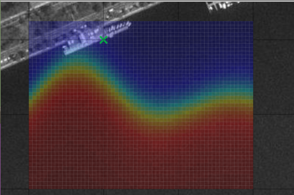
Figure 1.1: Ocean Front Estimation: An autonomous vehicle with a temperature sensor is used to estimate the dynamic properties of an ocean front, separating two water bodies of different temperatures, indicated by the color shading. The front is dynamic, and the objective is to estimate the parameters in an analytical model of the temperature versus time and location
A summary of today's topics:
- Migration of single-vehicle simulation to multi-vehicle field tests
- Proper operation on the river - OpRegion and CollisionAvoidance behaviors
- Sharing sensor information between vehicles for front estimation
- Preparing for the final in-water competition
2 Preliminaries
Make Sure You Have the Latest Updates [top]
Always make sure you have the latest code:
  $ cd moos-ivp
  $ svn update
And rebuild if necessary:
  $ ./build-moos.sh
  $ ./build-ivp.sh
Make Sure Key Executables are Built and In Your Path [top]
This lab does assume that you have a working MOOS-IvP tree checked out and installed on your computer. To verify this make sure that the following executables are built and findable in your shell path:
  $ which MOOSDB
  /Users/you/moos-ivp/bin/MOOSDB
  $ which pHelmIvP
  /Users/you/moos-ivp/bin/pHelmIvP
If unsuccessful with the above, return to the steps in Lab 1:
http://oceanai.mit.edu/ivpman/labs/machine_setup?
Where to Build and Store Lab Missions [top]
As with previous labs, we will use your version of the moos-ivp-extend tree, which by now you should have re-named something like moos-ivp-janedoe, where your email may be janedoe@mit.edu. In this tree, there is a missions folder:
  $ cd moos-ivp-janedoe
  $ ls
  CMakeLists.txt  bin/            build.sh*       docs/           missions/       src/
  README          build/          data/           lib/            scripts/
For each distinct stage in this lab, there should be a corresponding subdirectory in a lab_18 sub-directory of the missions folder, typically with both a .moos and .bhv configuration file.
Documentation Conventions [top]
To help distinguish between MOOS variables, MOOS configuration parameters, and behavior configuration parameters, we will use the following conventions:
- MOOS variables are rendered in green, such as IVPHELM_STATE, as well as postings to the MOOSDB, such as DEPLOY=true.
- MOOS configuration parameters are rendered in blue, such as AppTick=10 and verbose=true.
- Behavior parameters are rendered in brown, such as priority=100 and endflag=RETURN=true.
More Resources [top]
- The slides from lecture "Writing Behaviors":
http://oceanai.mit.edu/2.680/docs/2.680-14-writing_behaviors_2019.pdf - The slides from lecture "Helm Optimization":
http://oceanai.mit.edu/2.680/docs/2.680-15-optimization_2019.pdf - The slides from lecture "Parameter Estimation":
http://oceanai.mit.edu/2.680/docs/2.680-16-param_estimation_2018.pdf - The IvP Behavior Utility Functions
http://oceanai.mit.edu/ivpman/help/bhv_functions - The IvPBuild Toolbox ZAIC documentation
http://oceanai.mit.edu/ivpman/chap/ivpbuild_zaics
3 Structure of the Lab and Goals
This lab with stretch over the last week of the class. Initially, you will work with your partner on developing a collaboration strategy and modify your sampling behaviors accordingly. Later, we will work on implementing your autonomy system on the Herons, and in the last session we will finish with a competition.
3.1 Front Estimation Baseline Mission [top]
The shoreside and vehicle configuration you should use as template for the frontal estimation problem is the same as in lab 17 and is available in the class repository:
   moos-ivp/ivp/missions-2680/lab_16_front_estimate_baseline/

   (lab_16 is not a typo - this lab happened to have different number previously)
To execute the template lawnmower survey missions with two vehicles, shown in Figure 3.1 and the shoreside community, use the command:
$ ./launch.sh 10
The baseline mission should look similar to the video posted at:
Figure 3.1: The Front Estimation Baseline mission includes two vehicles each executing a lawnmower pattern at right angles to each other, periodically sampling the water temperature. video:(0:48): https://vimeo.com/92685133
This default mission also includes two other launch scripts, launch_vehicle.sh and launch_shoreside.sh. For this lab, you will be using launch_vehicle.sh or a modified version of it to launch each vehicle separately.
$ ./launch_vehicle.sh
3.2 Scoring [top]
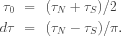
The scoring will be based on the RMS error and the elapsed time of the survey, using the following algorithm:

where  is the RMS error of the model parameters, and
  is a time penalty factor,
3.3 Communications [top]
For this lab, the communications between vehicles will be unlimited in size and frequency. The maximum message range will be set to 100m. The configuration block for meta_shoreside.moos is as follows:
 //--------------------------------------------------
 // uFldNodeComms Configuration Block

 ProcessConfig = uFldNodeComms
 {
   AppTick       = 2
   CommsTick     = 2

   comms_range          = 100
   critical_range       = 25
   min_msg_interval     = 0       // Unlimited frequency
   max_msg_length       = 0       // Unlimited length
   view_node_rpt_pulses = true
 }
4 Application Topology, Comms and Operation Area
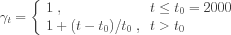
In this lab, although we will be working from the MIT Sailing Pavilion with physical platforms, the application topology is identical to the in-class simulations and competitions. A single shoreside computer will both serve as broker to the inter-vehicle communications and provide the simulated environmental sensor.
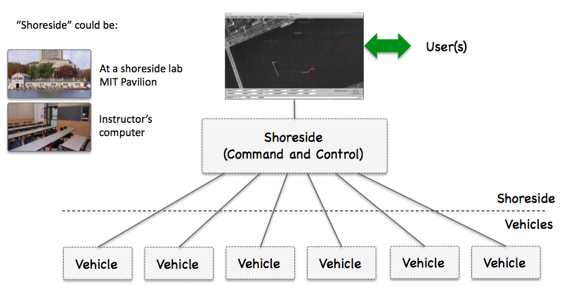
Figure 4.1: The Vehicle / Shoreside Topology
The baseline mission is in:
moos-ivp/ivp/missions-2680/lab_16_front_estimate_baseline/
It is configured with three vehicle communities in simulation. Because we will be running on the real vehicles rather than in simulation, a number of changes are necessary. Part of your assignment includes the conversion of this mission to a vehicle mission in your own tree(s). To do this we recommend that you create a launch_fld_vehicle.sh script, meta_fld_vehicle.moos and meta_fld_vehicle.bhv to your mission directory. Below are the changes that should be incorporated into these files from the baseline.
Modifications to the launch_vehicle.sh script [top]
- The vehicle script must not try to launch the shoreside.
- Modify the script so that you can reliably launch each vehicle for your mission, this may mean creating two separate scripts or adding command-line switches.
- It is convenient to retain the original launch script and meta files to maintain simulation ability. The new launch script can have a name like launch_vehicle_fld.sh (or alternatively could be a command-line switch to the launch_vehicle.sh script).
- Use the alpha_kayak launch scripts from Lab 16 as a guide to run on the PABLO unit, connected to the actual vehicle. Be sure to remove any multicast references in any pShare or uFldShoreBroker configurations. To reiterate from Lab 16, the launch script will allow you to set the IP address of the shoreside computer and the IP address of the vehicle.
- Remove all references to MOOS Time Warp when launching against the actual hardware.
Modifications to the meta_vehicle.moos and plugs [top]
- It is convenient to copy the meta_vehicle.moos to create meta_fld_vehicle.moos for deploying on actual hardware (see above).
- Be sure to remove any uSimMarine entries if found in the pAntler block and the associated plug include.
- Make sure iM200 is present in the pAntler block and the associated #include plug_iM200 statement.
- Copy plug_iM200.moos from Lab 16 into your working folder if needed.
- Verify that the shoreside IP address is being passed to uFldNodeBroker. If necessary, copy the uFldNodeBroker plug from Lab 16. This line should appear in the plug:
TRY_SHORE_HOST = pshare_route=$(SHORE_IP):$(SHORE_LISTEN)
- Verify that SHORE_IP and SHORE_LISTEN are defined in the launch script and are pushed through by nsplug.
The launch_shoreside.sh script [top]
- pHostInfo will need to have your IP address explicitly defined using HOSTIP_FORCE. Copy the contents of plug_pHostInfo.moos directly into the shoreside mission file. (instead of loading it through a plug). Set the following line:
DEFAULT_HOSTIP = $(HOSTIP_FORCE)
- Verify that HOSTIP_FORCE is defined in the launch script and is pushed through by nsplug.
Modifications to the meta_vehicle.bhv for River Operation [top]
- Your vehicles must utilize the BHV_OpRegion behavior to keep the vehicles from straying out of the operation area. See the documentation for this behavior. It also provides information about how far the vehicle presently is from the op region in terms of time and distance. It is recommended that if your vehicle gets too close to the op region boundary that you take corrective action. The OpRegion behavior shuts down the helm (sits dead in the water) when/if it violates the op region constraint.
- Your vehicle must also utilize the BHV_AvoidCollision to prevent damage to vehicles due to collisions.
4.1 Operation Area [top]
Due to Wi-Fi coverage constraints, and to keep our robots within eyesight and easy reach from the shore, the operation area is defined as in the BHV_OpRegion block of meta_vehicle.bhv in the baseline mission. This region is the polygon shown by the six vertices in Figure 3.1. Copy this block over into your behavior file as-is and set the flag OPREGION=true in your meta_vehicle.bhv file:
 initialize   OPREGION = true

 Behavior = BHV_OpRegion
 {
   name      = opregion
   pwt       = 100
   condition = MODE==ACTIVE
   condition = OPREGION=true

              polygon = pts={-50,-40 : 100,20 : 180,20 : 180,-200 : -50,-200 : -100,-75}
   trigger_entry_time = 1
   trigger_exit_time  = 1
         visual_hints = edge_size=1, vertex_size=2
 }
4.2 Collision Avoidance [top]
To prevent damage to vehicles, we also ask that you include the collision avoidance in your vehicle behavior file. Copy the Behavior=BHV_AvoidCollision block from the baseline meta_vehicle.bhv into your behavior file. The following block should be added to your code:
 initialize   AVOID   = true

 //------------------------------------------------
 Behavior = BHV_AvoidCollision
 {
   name       = avdcollision_
   pwt        = 200
   condition  = AVOID = true
   updates    = CONTACT_INFO
   endflag    = CONTACT_RESOLVED = $[CONTACT]
   templating = spawn

                contact = to-be-set
       on_no_contact_ok = true
            extrapolate = true
                  decay = 30,60

         pwt_outer_dist = 50
         pwt_inner_dist = 20
         completed_dist = 75
      min_util_cpa_dist = 8
      max_util_cpa_dist = 25
              pwt_grade = linear
    bearing_line_config = white:0, green:0.65, yellow:0.8, red:1.0
 }
5 Front Estimation
5.1 Front Model [top]
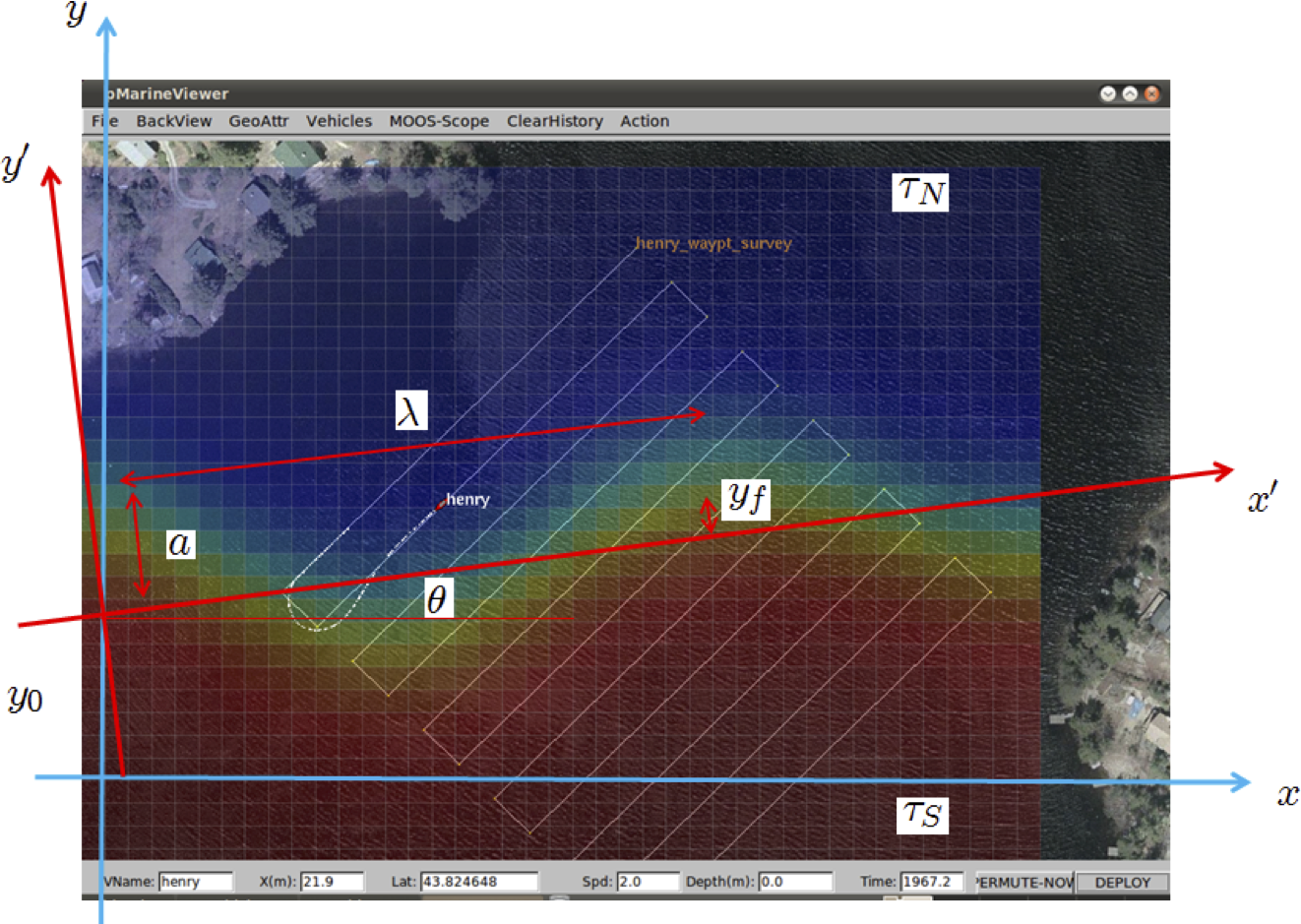
Figure 5.1: Ocean Front Estimation: The temperature field is parameterized by an analytical model with 9 parameters. In addition to the geometrical parameters shown here, the parameters include the temporal period T, the length scale of the frontal gradient,  , and the propagation decay
The temperature field is modeled by an analytical function, defined as follows.
The coordinate system aligned with the front, shown in Figure 5.1 is defines as
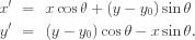
The position of the center of the front in the front coordinate system is

where  is the wavenumber and
  is the radial frequency. The temperature field is then given by

where
The sensor model used by the vehicles is uFldCTDSensor which simulates the front and takes virtual measurements of the associated temperature field using the class CFrontSim. The sensor simulator is operated in the shoreside community. A vehicle requests the measurement by publishing the variable UCTD_SENSOR_REQUEST to the MOOSDB with the value vname=my_auv. In the template configuration the measurement request are scheduled by the process uTimerScript, with the sampling period set in the plug plug_uTimerScript.moos. When you develop your behavior you may use the scheduler or directly issue the requests from your behavior. The measurement is returned in the MOOS variable UCTD_MSMNT_REPORT:
UCTD_MSMNT_REPORT = vname=my_auv,utc=123456789.0,x=123.45,y=345.67,temp=22.34
You control the dynamics of the frontal simulator by setting the ground truth parameters in the plug plug_uFLDCTDSensor.moos:
 // uFldCTDSensor configuration block from plugin

 ProcessConfig = uFldCTDSensor
 {
   AppTick   = 3
   CommsTick = 3

    // Configuring Model of Dynamic Front
   xmin  = 0;
   xmax  = 500;
   ymin  = -400;
   ymax  =  0;

   offset = -100;              // y_0
   angle  = 12;                // front angle theta
   amplitude = 20;            // spatial amplitude a
   period = 350;              // temporal period T
   wavelength = 200;          // spatial wavelength lambda
   alpha = 500;               // spatial 1/e length scale alpha
   beta = 20;                 // length scale of frontal gradient beta
   temperature_north = 20;    // temperature North of front
   temperature_south = 24;    // temperature South of front
   sigma = 0.01;              // standard deviation of gaussian sensor noise
 }
5.2 Parameter Estimation [top]
On your vehicle you will run the parameter estimation process pFrontEstimate which subscribes to the sensor report. It must be configured with the minimum and maximum of all the frontal model parameters in the plug plug_pFrontEstimate.moos:
 ProcessConfig = pFrontEstimate
 {
   AppTick    = 4
   CommsTick  = 4

   vname = $(VNAME)
   temperature_factor = $(COOL_FAC)
   cooling_steps = $(COOL_STEPS)
   min_offset = -120;
   max_offset = -60;
   min_angle = -5;
   max_angle = 15;
   min_amplitude = 0;
   max_amplitude = 50;
   min_period = 200;
   max_period = 600;
   min_wavelength = 100;
   max_wavelength = 500;
   min_alpha = 500;
   max_alpha = 500;
   min_beta = 10;
   max_beta = 30;
   min_T_N = 15;
   max_T_N = 25;
   min_T_S = 20;
   max_T_S = 30;
   concurrent = true           // Flag controlling whether the
                               // annealing is performed concurrently
                               // with survey.
   adaptive = true             // Uses adaptive simulated annealing,
                               // where the parameter search interval
                               // reduced proportionally to temperature
 }
The cooling parameters are set in the launch script or on the command line. Note the parameter concurrent which is used to control whether the annealing is performed concurrently with the survey. This feature can be used to save time, but it has to be used with care, in particular if combined with fast cooling (cooling_steps small), because the parameters may 'freeze' before the survey reaches the areas which provide the most information.
Another important parameter is adaptive, which controls whether adaptive simulated annealing (ASA). In ASA, the parameter search intervakl is shunk around the current estimate, proportionally to the cooling temperature  . It yields a more robust estimate because large jumps are avoided once a good solution is arrived at, but the cooling factor becomes more critical. Thus, if k is chosen too small, you may get caught in a false, local minimum.
Note also that you may 'fix' one or more variables by simply setting the min and max values equal to the true value. This is useful for determining the utility of a survey strategy for determining a specific parameter or the coupling between a couple of parameters, as you will be ask do do in the assignments.
The measurement collection and the parameter estimation is initiated when the survey flag is set in the MOOSDB:
SURVEY_UNDERWAY = true
which must be set by the survey behavior. You can see how this is done with the active_flag in the meta file for the vehicle helm, meta_vehicle.bhv:
 // Helm Behavior file

 initialize   DEPLOY  = true
 initialize   RETURN  = false
 initialize   STATION_KEEP = false
 initialize   SURVEY  = true
 initialize   AVOID   = true
 initialize   SURVEY_UNDERWAY = false

 set MODE = ACTIVE {
   DEPLOY = true
 } INACTIVE

 set MODE = RETURNING {
   MODE = ACTIVE
   RETURN = true
 }

 set MODE = SURVEYING {
   MODE = ACTIVE
   SURVEY = true
   RETURN = false
 }

 //----------------------------------------------
 Behavior = BHV_Waypoint
 {
   name         = waypt_survey
   pwt          = 100
   condition    = MODE==SURVEYING
   perpetual    = true
   updates      = SURVEY_UPDATES
   activeflag   = SURVEY_UNDERWAY = true
   inactiveflag = SURVEY_UNDERWAY = false
   endflag      = RETURN = true

           lead = 8
    lead_damper = 1
          speed = 2.0   // meters per second
         radius = 8.0
         points = format=lawnmower, label=dudley_survey, x=$(SURVEY_X), y=$(SURVEY_Y),
                  width=$(WIDTH), height=$(HEIGHT), lane_width=$(LANE_WIDTH),
                  rows=north-south, degs=$(DEGREES)
   visual_hints = nextpt_color=red, nextpt_lcolor=khaki
   visual_hints = vertex_color=yellow, line_color=white
   visual_hints = vertex_size=2, edge_size=1
 }
5.2.1 Adding Measurements from Collaborator [top]
In this lab you have the possibility of adding measurements made by another vehicle. The class used for each measurement has the structure
 class CMeasurement
 {
  public:
   double t;
   double x;
   double y;
   double temp;
 };
where t is the time of the measurement, x,y is the location, and temp is the temperature. This class is defined in the lib_henrik_util library of the moos-ivp tree. When a measurement report is received in the moos variable UCTD_SENSOR_REPORT, it is parsed into a measurement by the function
CMeasurement CSimAnneal::parseMeas(string report)
returning an associated member of the measurement class. The process pFrontEstimate uses this function whenever a new measurement is coming in, and is then added to the current measurement vector by the function
void CSimAnneal::addMeas(CMeasurement new_meas)
To add measurements made by another vehicle, you will have to create a message which transmits one or more measurements and pass them on to the parameter estimation process. It is up to you how to do that. One way is to pass the measurements as UCTD_SENSOR_REPORT to the collaborator vehicle, but you may instead want to make new message with a vector of measurements, and then code them each into the UCTD_SENSOR_REPORT format on the receiving vehicle.
6 Lab Assignment
6.1 Preparing for the Competition [top]
6.1.1 Vehicle Name [top]
Configure your autonomy system such the the name of your vehicle is your first name. This will avoid conflicts in the dual-vehicle survey, and allow us to keep better track of your scores.
6.1.2 pHelmIvP Configuration [top]
Ensure your behavior configuration incorporates the bounding box using the OpRegion behavior, to ensure the Heron is not run through the locks and out into the Atlantic, or run it into the dock or the Longfellow Bridge. Consider using the recently augmented OpRegion that has the optional parameter soft_poly_breach=true, which will allow you to command your vehicle to re-start when/if it goes out of the operation region. Also, ensure the BHV_AvoidCollision behavior is properaly configured and enabled so your two vehicles don't run into each other.
6.1.3 Configure Parameter Estimation [top]
Configure the parameter estimator process pFrontEstimate. As noted in the previous lab, the parameter alpha is very difficult to estimate with the small survey area we have, and the scores were highly dependent on the mismatch in the estimate of this parameter. For this lab the value will be fixed to 500. Make a few trial runs with the two vehicles to familiarize yourself with the performance.
6.1.4 Simultaneous Surveying [top]
Implement your adaptive sampling behavior, or if you have an improved version, use that. Then work with your partner to launch both of your vehicles with a common shoreside and run simultaneous missions to ensure that the bounding-box and collision avaoidance behaviors are properly configured.
6.1.5 Measurement Data Sharing [top]
Modify the pFrontEstimate process to allow the occasional addition of measurement data and incorporate them in the annealing. Test this out with the template surveys.
6.1.6 Adaptive Collaborative Survey [top]
As the final step, modify you behaviors and processes to execute a collaborative survey. You will be able to communicate with unlimited frequency and bandwidth when the two vehicles are within communication range.
6.2 Competition Dates [top]
The final in-water competition will be held at the Sailing Pavilion during the last week of classes, Mon-Thur, May 14-16, 2019. All teams should prepare to run their vehicles for a minimum of two runs. One successful run is mandatory to receive credit for the lab, and two runs are required to receive an A for the lab. Student teams will receive their final ranking after each team has completed at least one run. Teams that complete two runs, with two distinct unknown fronts, will automatically rank higher than teams completing only one run.
It is highly recommended that each team gets as much in-water practice as possible leading up to the final competition. A good goal during the run-up preparations would be to have your two vehicles running with some version of your behaviors functional and reporting a score to the shoreside. If this is not possible, try to test one vehicle with a simulated partner vehicle instead.
Good Luck Everyone !!!!!
Document Maintained by: mikerb@mit.edu
Page built from LaTeX source using texwiki, developed at MIT. Errata to issues@moos-ivp.org. Get PDF