Lab 17 - Collaborative Autonomous Front Estimation
Maintained by: mikerb@mit.edu  Get PDF
1 Overview and Objectives
2 Preliminaries
3 Structure of the Lab and Goals
3.1 The Front Estimation Baseline Mission
3.2 Scoring and the pGradeFronteEstimate Application
4 Front Estimation
4.1 The Front Model and the uFldCTDSensor Application
4.2 Parameter Estimation
4.3 Assignment Section A
4.3.1 Annealing Schedule
4.3.2 Parameter Sensitivity
4.3.3 Dynamic Front
4.3.4 Survey Pattern
4.3.5 Multi-parameter Estimation
4.4 Assignment Section B
4.4.1 Adaptive Sampling Behavior
4.4.2 Collaborative Sampling
5 Sharing Sensor Measurements
5.1 Inter-Vehicle Messaging
5.2 Make Your Own pFrontEstimate App
5.3 Share Sensor Information From Your pFrontEstimate App
5.3.1 Identifying Sensor Data to be Shared
5.3.2 Creating an Outgoing Message for Shared Data
5.3.3 Testing the Communications
5.4 Messaging with Limitations on Comms Range
6 Mission Test Parameters and Ranges
1 Overview and Objectives
In the previous labs we have focused on remote sensing techniques for detecting, classifying and locating (DLT) sea-bed hazards. Another common application of autonomous vehicles involves the measurement of oceanographic properties using physical, chemical or biological sensors mounted on the vehicles. For this problem the sensors provide point measurements at the location of the AUV. A common problem in coastal oceanography is the spatial and temporal characterization of a front separating water masses of different temperature, as shown in Fig.~ 1.1. Only in a few pathological cases the front will be stationary in space and time, and in general the measurements will have to support the estimation of the dynamic properties of the front. This problem is complicated by the space-time aliasing inherent to the sampling of a dynamic field by a point sensor with finite mobility. In other words, an AUV with a temperature sensor does not provide a synoptic measurement of the temperature field, and a change observed between two measurements may not be directly associated with a spatial or a temporal change.

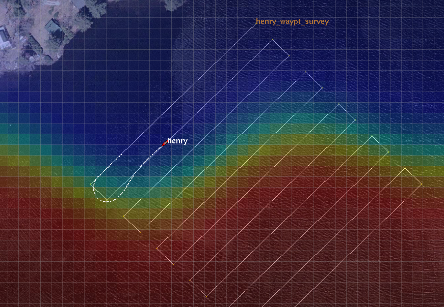
Figure 1.1: Ocean Front Estimation: An autonomous vehicle with a temperature sensor is used to estimate the dynamic properties of an ocean front, separating two water bodies of different temperatures, indicated by the color shading. The front is dynamic, and the objective is to estimate the parameters in an analytical model of the temperature versus time and location
To break this ambiguity one must in general apply a parametric model of the oceanographic phenomenon, and then design a survey which provides a reliable estimate of the parameters. This approach first of all requires that the model makes sense physically, and the most robust approach is to choose a model which is consistent with the physics of the problem. A suite of such oceanographic models exist, but their use is beyond the scope of this class. Instead we will use an analytical model for the temperature field, but the principles of the oceanographic sampling problem are the same. Thus the survey selected for the measurements by the AUV must be chosen in such a way that the measurements provide an estimate which is unambiguous in space and time. This in general is a complex problem with no unique solution, but some general guidelines exist for the survey:
- The survey must focus on the areas that provide the most information about the model parameters, in general translating into a strategy of concentrating the survey in areas of strong gradients.
- While focusing most effort in areas of strong variability, the geographical region of interest must be adequately covered.
- The survey should be designed to optimally un-couple the parameters, i.e. avoid patterns which provide information that is ambiguous in the parameters.
A summary of today's topics:
- Front estimation first using a static pre-determined mission
- Behavior-writing for adaptive sampling and front estimation
- Simulated Annealing for front estimation
- In-water exercises in autonomous collaborative front estimation
2 Preliminaries
Make Sure You Have the Latest Updates [top]
Always make sure you have the latest code:
  $ cd moos-ivp
  $ svn update
And rebuild if necessary:
  $ ./build-moos.sh
  $ ./build-ivp.sh
Make Sure Key Executables are Built and In Your Path [top]
This lab does assume that you have a working MOOS-IvP tree checked out and installed on your computer. To verify this make sure that the following executables are built and findable in your shell path:
  $ which MOOSDB
  /Users/you/moos-ivp/bin/MOOSDB
  $ which pHelmIvP
  /Users/you/moos-ivp/bin/pHelmIvP
If unsuccessful with the above, return to the steps in Lab 1:
http://oceanai.mit.edu/ivpman/labs/machine_setup?
Where to Build and Store Lab Missions [top]
As with previous labs, we will use your version of the moos-ivp-extend tree. In this tree, there is a missions folder:
  $ cd moos-ivp-extend
  $ ls
  CMakeLists.txt  bin/            build.sh*       docs/           missions/       src/
  README          build/          data/           lib/            scripts/
For each distinct stage in this lab, there should be a corresponding subdirectory in a lab_16 sub-directory of the missions folder, typically with both a .moos and .bhv configuration file.
Documentation Conventions [top]
To help distinguish between MOOS variables, MOOS configuration parameters, and behavior configuration parameters, we will use the following conventions:
- MOOS variables are rendered in green, such as IVPHELM_STATE, as well as postings to the MOOSDB, such as DEPLOY=true.
- MOOS configuration parameters are rendered in blue, such as AppTick=10 and verbose=true.
- Behavior parameters are rendered in brown, such as priority=100 and endflag=RETURN=true.
More Resources [top]
- The slides from lecture "Writing Behaviors":
http://oceanai.mit.edu/2.680/docs/2.680-14-writing_behaviors_2021.pdf - The slides from lecture "Helm Optimization":
http://oceanai.mit.edu/2.680/docs/2.680-15-optimization_2021.pdf - The slides from lecture "Parameter Estimation":
http://oceanai.mit.edu/2.680/docs/2.680-16-param_estimation_2020.pdf - The IvP Behavior Utility Functions
http://oceanai.mit.edu/ivpman/help/bhv_functions - The IvPBuild Toolbox ZAIC documentation
http://oceanai.mit.edu/ivpman/chap/ivpbuild_zaics
3 Structure of the Lab and Goals
This lab with stretch over four lab sessions. In the first session, you will use a scripted lawn-mower survey to collect the data for the parameter estimation, and use it to develop an understanding of the coupling between the model parameters and the effects of changes in the survey design.
In the next part, the goal will be to write a couple of intermediate simple behaviors. In the final part you will, based on the experience gained in the first parts, design your own IvP behavior for estimating the model parameters in the shortest amount of time.
You will be provided a MOOS module for performing the parameter estimation using simulated annealing, but you have to select the control parameters for the algorithm, most importantly those controlling the 'cooling' schedule. You will be able to modify the front model as you see fit to test your behavior.
During the last lab session, we will run a blind test of your algorithm and behavior, where we control the front simulator and your vehicle will have to perform its survey and determine a parameter estimate. The grading will be based on a score that is inversely proportional to the parameter estimation error and the time for the survey and the parameter estimation.
3.1 The Front Estimation Baseline Mission [top]
Before jumping into the assignments following, you may want to familiarize yourself with the baseline mission configuration. The shoreside and vehicle configuration you should use as template for the frontal estimation problem is available in the class repository:
moos-ivp/ivp/missions-2680/lab_16_front_estimate_baseline_2021/
Make a copy of this mission into your moos-ivp-extend directory. The baseline mission may be launched by:
$ ./launch.sh 15 --cool=50 --angle=0 -a --one
where the switches represent:
- warp: Time warp factor as usual. You should be able to do at least 10 here.
- cool: The cooling factor k applied to the Boltzman probability in the simulated annealing,
 .
.
- angle: The angle of the survey legs. 0 yields vertical survey legs,
 horizontal legs.
- -uc: If this switch is set, the annealing will happen non-concurrently with your survey, waiting to add measurements until you return the vehicle.
- -a: Use adaptive simulated annealing, reducing the parameter search intervals with cooling.
- --one: Launch only one vehicle. The default is two vehicles.
The launch script is set to use the concurrent setting by default (add new measurements to the annealer as they arrive). To run the annealer not concurrent, use flag -uc.
The baseline mission should look similar to the video posted at:
Figure 3.1: The Front Estimation Baseline mission includes two vehicles each executing a lawnmower pattern at right angles to each other, periodically sampling the water temperature. video:(0:48): https://vimeo.com/92685133
3.2 Scoring and the pGradeFronteEstimate Application [top]
The scoring will be based on the RMS error and the elapsed time of the survey, using the following algorithm:

where  is the RMS error of the model parameters, and
  is a time penalty factor,
The pGradeFrontEstimate Application [top]
The grading is automatically handled by the pGradeFrontEstimate running in the shoreside community. When a report is received from one of the vehicles, this app will produce a report, similar to the below example, to the appcast output in pMarineViewer or the uMAC windows.
 ===================================================================
 pGradeFrontEstimate shoreside                              0/0(762)
 ===================================================================
 GradeFrontEstimate
 ------------------------
 ===================
 Report from archie
 ===================
 Error        0.165876
 Elapsed time 574.226
 Score        524.932
 Parameter estimates
 ===================
 Offset     -88.1533 Actual -90
 Angle      3.28807 Actual 5
 Amplitude  20.139 Actual 20
 Period     203.925 Actual 200
 Wavelength 228.095 Actual 200
 Alpha      499.832 Actual 400
 Beta       15.6445 Actual 20
 Temp_North 20.1557 Actual 20
 Temp_South 24.8385 Actual 25
The pGradeFrontEstimate application receives "ground truth" from the incoming MOOS variable UCTD_TRUE_PARAMETERS, published by the uFldCTDSensor. It receives a report from one of the vehicles in the form of the variable UCTD_PARAMETER_ESTIMATE, shared from one of the vehicles to the shoreside. An example estimate:
 UCTD_PARAMETER_ESTIMATE = vname=archie,offset=-88.15331,angle=3.28807,amplitude=20.13901,
                           period=203.92525,wavelength=228.09496,alpha=499.83167,
                           beta=15.64447,tempnorth=20.15573,tempsouth=24.83851
4 Front Estimation
4.1 The Front Model and the uFldCTDSensor Application [top]
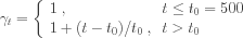
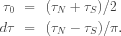
The temperature field is modeled by an analytical function, defined as follows. The coordinate system aligned with the front, shown in Figure 4.1 is defines as
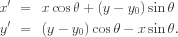
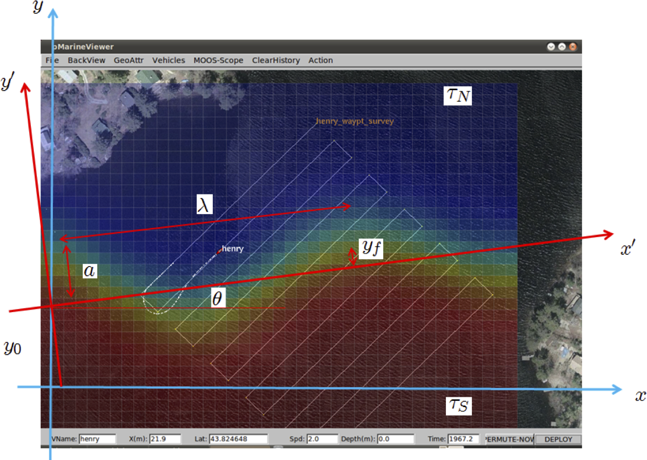
Figure 4.1: Ocean Front Estimation: The temperature field is parameterized by an analytical model with 9 parameters. In addition to the geometrical parameters shown here, the parameters include the temporal period T, the length scale of the frontal gradient,  , and the propagation decay
The position of the center of the front in the front coordinate system is

where  is the wavenumber and
  is the radial frequency. The temperature field is then given by

where
The uFldCTDSensor Application [top]
The sensor model used by the vehicles is uFldCTDSensor which simulates the front and takes virtual measurements of the associated temperature field using the class CFrontSim. The sensor simulator is operated in the shoreside community. A vehicle requests the measurement by publishing the variable UCTD_SENSOR_REQUEST to the MOOSDB with the value vname=my_auv. In the template configuration the measurement requests are scheduled by the process uTimerScript, with the sampling period set in the file plug_uTimerScript.moos. When you develop your behavior you may use the scheduler or directly issue the requests from your behavior. The measurement is returned in the MOOS variable UCTD_MSMNT_REPORT with the content
UCTD_MSMNT_REPORT = vname=my_auv,utc=123456789.0,x=123.45,y=345.67,temp=22.34
You control the dynamics of the frontal simulator by setting the ground truth parameters in the file plug_uFldCTDSensor.moos:
 ProcessConfig = uFldCTDSensor
 {
   AppTick   = 3
   CommsTick = 3

    // Configuring Model of Dynamic Front
   xmin  = 0;
   xmax  = 500;
   ymin  = -400;
   ymax  =  0;

   offset = -90;              // y_0
   angle  = 5;                // front angle theta
   amplitude = 20;            // spatial amplitude a
   period = 200;              // temporal period T
   wavelength = 200;          // spatial wavelength lambda
   alpha = 400;               // spatial 1/e length scale alpha
   beta = 20;                 // length scale of frontal gradient beta
   temperature_north = 20;    // temperature North of front
   temperature_south = 25;    // temperature South of front
   sigma = 0.01;              // standard deviation of Gaussian sensor noise
 }
To get a visual idea of how the front varies with some of these parameters, see the video or figure below. Three fronts are rendered. The first has the parameters shown in the above listing. The variations are shown with by changing the parameters indicated:
Figure 4.2: Variations on the ground truth thermal front as produced by the uFldCTDSensor application and rendered in pMarineViewer with a grid structure produced by pFrontGridRender. The first frame shows the front using the default parameters. The second front reflects a change of angle to 45 degrees. The third front reflects a change in amplitude to 35, and period to 100. video:(0:34): https://vimeo.com/92666130
4.2 Parameter Estimation [top]
On your vehicle you will run the parameter estimation process pFrontEstimate which subscribes to the sensor report. It must be configured with the minimum and maximum of all the frontal model parameters in the file plug_pFrontEstimate.moos:
 ProcessConfig = pFrontEstimate
 {
   AppTick    = 4
   CommsTick  = 4

   vname = $(VNAME)
   temperature_factor = $(COOL_FAC)
   cooling_steps = $(COOL_STEPS)
   min_offset = -120;
   max_offset = -60;
   min_angle = -5;
   max_angle = 15;
   min_amplitude = 0;
   max_amplitude = 50;
   min_period = 200;
   max_period = 600;
   min_wavelength = 100;
   max_wavelength = 500;
   min_alpha = 500;
   max_alpha = 500;
   min_beta = 10;
   max_beta = 30;
   min_T_N = 15;
   max_T_N = 25;
   min_T_S = 20;
   max_T_S = 30;
   concurrent = $(CONCURRENT)  // Flag controlling whether the
                               // annealing is performed concurrently
                               // with survey.
   adaptive = $(ADAPTIVE)      // Uses adaptive simulated annealing,
                               // where the parameter search interval
                               // reduced proportionally to temperature
 }
The cooling parameters are set in the launch script or on the command line. Note the parameter concurrent which is used to control whether the annealing is performed concurrently with the survey. This feature can be used to save time, but it has to be used with care, in particular if combined with fast cooling (cooling_steps small), because the parameters may 'freeze' before the survey reaches the areas which provide the most information.
Another important parameter is adaptive, which controls whether adaptive simulated annealing (ASA) is used. In ASA, the parameter search interval is shrunk around the current estimate, proportionally to the cooling temperature  . It yields a more robust estimate because large jumps are avoided once a good solution is arrived at, but the cooling factor becomes more critical. Thus, if k is chosen too small, you may get caught in a false, local minimum.
Note also that you may 'fix' one or more variables by simply setting the min and max values equal to the true value. This is useful for determining the utility of a survey strategy for determining a specific parameter or the coupling between a couple of parameters, as you will be asked to do in the assignments.
The measurement collection and the parameter estimation is initiated when the survey flag is set in the MOOSDB:
SURVEY_UNDERWAY = true
which must be set by the survey behavior. You can see how this is done with the active_flag in the meta file for the vehicle helm, meta_vehicle.bhv:
 //---------------------------------------------------
 // Helm Behavior file

 initialize   DEPLOY  = true
 initialize   RETURN  = false
 initialize   STATION_KEEP = false
 initialize   SURVEY  = true
 initialize   AVOID   = true
 initialize   SURVEY_UNDERWAY = false

 set MODE = ACTIVE {
   DEPLOY = true
 } INACTIVE

 set MODE = RETURNING {
   MODE = ACTIVE
   RETURN = true
 }

 set MODE = SURVEYING {
   MODE = ACTIVE
   SURVEY = true
   RETURN = false
 }

 //----------------------------------------------
 Behavior = BHV_Waypoint
 {
   name         = waypt_survey
   pwt          = 100
   condition    = MODE==SURVEYING
   perpetual    = true
   updates      = SURVEY_UPDATES
   activeflag   = SURVEY_UNDERWAY = true            <-- begin measure/estimate
   inactiveflag = SURVEY_UNDERWAY = false
   endflag      = RETURN = true

           lead = 8
    lead_damper = 1
          speed = 2.0   // meters per second
         radius = 8.0
         points = format=lawnmower, label=dudley_survey, x=$(SURVEY_X), y=$(SURVEY_Y),
                  width=$(WIDTH), height=$(HEIGHT), lane_width=$(LANE_WIDTH),
                  rows=north-south, degs=$(DEGREES)
   visual_hints = nextpt_color=red, nextpt_lcolor=khaki
   visual_hints = vertex_color=yellow, line_color=white
   visual_hints = vertex_size=2, edge_size=1
 }
When you write your own behavior in the second part of the assignment you will have to configure it in a similar way.
4.3 Assignment Section A [top]
In the first part of the assignment, we will focus on developing a fundamental understanding of the front model parameterization and the role of the survey pattern in isolating or coupling the various parameters. Also, we are using a simulated annealing algorithm for the parameter estimation, and we have to make sure we choose the cooling schedule properly to arrive at a good parameter estimate. We will try to achieve that through a sequence of exercises using the template configuration in missions-2680/lab_16_front_estimate_baseline. The deliverable for this lab should be a quick write up for each of five subsections below to show that you've done the work and have some intuitive sense of what is going on in each of the steps.
The lab is open-ended and unstructured, and you should use your own intuition for this 'learning phase':
- Note that there is no unique solution, so use your common sense in your analysis.
- The parameter settings in the following exercises are only suggestions. If you see something interesting, choose your own settings.
- Also, do not base your discussion on a single survey run, the score may vary significantly due to the stochastic nature of the estimator. You can do this by simply re-deploying the vehicle.
4.3.1 Annealing Schedule [top]
For this exercise we will initially fix some of the parameters, and make the front quasi-stationary. Set the following uFldCTDSensor parameters in corresponding plug file, plug_uFldCTDSensor.moos:
   alpha = 500
   beta = 20
   angle = 5
   period = 196
First launch the shoreside, invoking:
$ ./launch_shoreside.sh
Then launch a vehicle, invoking
$ ./launch_vehicle.sh
This default survey will run with angle=0, cool=50, and concurrent="true". Change the cooling factor to see what happens.
The flags for launch_vehicle.sh are the same as for launch.sh, and it will take --vname=VNAME as an additional argument. Note that you can re-launch the vehicle without restarting the shoreside.
Next, open up the search interval for the parameter alpha to the interval [300,800]. Do you observe a difference in performance? Explain.
Also, try to run the annealer after all measurements are collected, by invoking the launch script command line option -uc. This will make pFrontEstimate parameter concurrent="false".
4.3.2 Parameter Sensitivity [top]
Fix all parameters except one, the wavelength, run several surveys and make a plot of the score versus estimated wavelength error.
4.3.3 Dynamic Front [top]
Repeat the exercise with two parameters unknown, the wavelength and the period. Add dynamics by setting period=200 with search interval [100,300]. Discuss the results.
4.3.4 Survey Pattern [top]
Repeat the survey with lawnmower angle settings of 225 and 270 degrees using: the following vehicle launch script parameter:
--angle=225
Also, try changing the survey lane width. Discuss your findings. You may want to focus on wavelength and period, fixing all other parameters. Which survey angle do you think best separates the two parameters? Is your expectation confirmed by the survey?
4.3.5 Multi-parameter Estimation [top]
Open up the search interval for all parameters.
4.4 Assignment Section B [top]
4.4.1 Adaptive Sampling Behavior [top]
In the second part of the assignment you should use your experience from the survey exercises to develop your own strategy for sampling the field and estimate the parameters as accurately as possible in the shortest amount of time, and build it into a new IvPHelm behavior, adapting to the measured temperature field.
Your behavior must perform both the search for the front and then survey it in an optimal manner. You may either write a single behavior doing both phases or you may set up the search and the mapping phases as separate modes. The objective is to get the smallest parameter error in the shortest amount of time.
The deliverable for this step is to run your vehicle code with on a shoreside computer that is run by one of the instructors. You will have two attempts of 7 minutes each (from deploy to report) to try to characterize the front, give a report, and get a score which will be recorded and compared to other members of the class.
4.4.2 Collaborative Sampling [top]
The next lab will consist of developing collaborative vehicle behaviors for front estimation on the river. As the last part of the assignment, make sure you've identified a lab partner, and together, speculate on how you would design a collaborative behavior strategy for reaching the objective. Discuss this with one of the instructors.
5 Sharing Sensor Measurements
A core goal of this lab is to enable the pair of deployed vehicles to share sensor information to allow each vehicle to use as much data collected from the other vehicle as possible. The annealing algorithm used by pFrontEstimate will accept time-stamped temperature measurements with x-y location. For the received measurements, the order and timing may matter depending on the annealer configuration, with later measurements at some point arriving too late after the annealer has settled on a solution. So sharing measurements sooner rather than later is preferred, but it is not that case that late shared measurements will hurt the solution. So the a good general strategy is to (a) share everything, (b) share as soon as possible. In this section we describe how to set up measurement messaging.
5.1 Inter-Vehicle Messaging [top]
Sharing sensor measurements between vehicles will use the uFlield tools similar to previous labs.
- A message is generated on the source vehicle, posted in the NODE_MESSAGE_LOCAL MOOS variable.
- This variable is shared to the shoreside from the vehicle. This sharing is already configured in the uFldNodeBroker config block in the vehicle .moos file.
- On the shoreside uFldNodeComms decides whether to pass the message to the destination vehicle base on configured constraints. In this lab, messages will only reach their destination vehicle if the two vehicles are less or equal to 100 meters.
- If the message reaches the destination vehicle, uFldMessageHandler will unpack the message and make the posting to the local MOOSDB. In our case the posting will be a sensor measurement shared from the collaborating vehicle.
Nearly all of this is already in place in the baseline mission. The message passing constructs on both the shoreside and vehicle communities are typically part of our style of mission configuration.
The primary task left to add in this lab, is to somehow receive our own sensor measurements and then share them to the other vehicle. This is discussed next. Since we are already receiving sensor measurements in pFrontEstimate, we recommend using this app to accomplish the sharing. But pFrontEstimate is part of the MOOS-IvP tree, so we will make a copy of this app that we can modify and put under our own version control.
5.2 Make Your Own pFrontEstimate App [top]
The pFrontEstimate app is part of the MOOS-IvP codebase, written by Prof. Schmidt. You can modify the code, but you can't check in changes since the MOOS-IvP codebase is read-only. The goal in this step is to make a copy of pFrontEstimate, and add it to your moos-ivp-extend tree where you can modify and check in your changes. We go through the steps below, from the perspective of Subversion, but the steps are similar for git.
Step 1: Copy the App [top]
First the app is copied to the home directory and then moved to your own tree:
   $ cd moos-ivp/ivp/src
   $ cp -rp pFrontEstimate ~/
   $ cd moos-ivp-extend/src
   $ mv pFrontEstimate .
Step 2: Put the app under version control [top]
   $ cd moos-ivp-extend/src
   $ svn add pFrontEstimate
   A         pFrontEstimate
   $ svn commit -m "added new app" pFrontEstimate
   Adding         pFrontEstimate
   Committing transaction...
   Committed revision 766.
Step 3: Add the new App to your build [top]
   $ cd moos-ivp-extend/src
   $ emacs -nw CMakeLists.txt

   add the line:
   ADD\_SUBDIRECTORY(pFrontEstimate)
   save the file
Eventually you will need to commit this change too.
Step 4: Modify your Shell Path if Necessary [top]
Once you build your augmented moos-ivp-extent tree, there will be two pFrontEstimate apps on your computer. Hereafter you will want to use yours. To do this, edit your .bashrc file and find the section where you set your shell path. Look for the below two lines among this group, and make sure the moos-ivp-extend bin directory is before the moos-ivp directory as below.
   PATH=$PATH:~/moos-ivp-extend/bin
   PATH=$PATH:~/moos-ivp/bin
After you have done all this (and built your new tree with your version of pFrontEstimate), verify that your new app is findable:
   $ which pFrontEstimate
   /Users/username/moos-ivp-extent/bin/pFrontEstimate
Or in Linux, slightly different:
   $ which pFrontEstimate
   /home/username/moos-ivp-extent/bin/pFrontEstimate
If you want, you can try which -a and you should see both binaries, in the proper order.
5.3 Share Sensor Information From Your pFrontEstimate App [top]
Now that you have your own pFrontEstimate app, you are free to extend it to suit your needs. The first suggestion is to use this app to share sensor measurement data. Although the purpose of this app is to receive censor data via the MOOS variable UCTD_MSMNT_REPORT, it is also a convenient spot to take the additional step of sharing this measurement data to the collaborating vehicle. There is no single right design for which app can do this (you could write your own additional MOOS app to handle this for example), but this approach seems convenient, so it will be described here.
5.3.1 Identifying Sensor Data to be Shared [top]
In the OnNewMail() function of (your) pFrontEstimate, incoming mail from the simulated CTD sensor arrives in the form:
UCTD_MSMNT_REPORT = vname=archie,utc=123456789.0,x=123.45,y=345.67,temp=22.34
The above sensor measurement was obtained by vehicle archie, indicated in the first field of the message. If the collaborating vehicle is betty, then we'd like to share this message to betty. However, we need to ensure that betty doesn't in turn share it back to archie, creating an endless loop of redundant data.
Once sharing is established, there will be two streams of sensor data, the organic data obtained from one's own sensor, and the shared data received from a collaborating vehicle. We need to ensure that each vehicle is only sharing its organic data. There a couple ways to do this:
Method 1: In the pFrontEstimate app, there already exists a member variable vname, holding the name of ownship. You can identify incoming shared data by checking the vname field in the incoming sensor report and compare against ownship. Archie will only share organic data, the reports with archie as the vehicle name. A reminder: the tokStringParse() function is particularly useful for grabbing a single field from a string like the measurement report string.
Method 2: Share all data received via UCTD_MSTMT_REPORT, but shared data is posted to the variable UCTD_MSMNT_REPORT_SHARED. The pFrontEstimate app will need to also register for this variable, and process the data the same way that UCTD_MSTMT_REPORT data is handled.
5.3.2 Creating an Outgoing Message for Shared Data [top]
Now that we know which sensor data will be shared, the next question is how. Per the discussion above, in Section 5.1, this will be done by (a) posting to NODE_MESSAGE_LOCAL, and (b) received using the uFldMessageHandler app on the receiving vehicle. The focus here is on how to compose an outgoing message:
UCTD_MSMNT_REPORT = vname=archie,utc=123456789.0,x=123.45,y=345.67,temp=22.34
This message will be sent by betty to archie, from with the pFrontEstimate app running on archie.
Recall from the Inter-vehicle messaging lab that we can easily create a syntactically correct NODE_MESSAGE by using the NodeMessage class. The below snippet of code is repeated for convenience from the uFldMessageHandler documentation.
  #include "NodeMessage.h"  // In the lib_ufield library

  string m_hostname;        // ownship name
  string m_dest_name;       // collaborator name
  string m_moos_varname;    // "UCTD_MSMNT_REPORT"
  string m_msg_contents;    // sensor report

  NodeMessage node_message;

  node_message.setSourceNode(m_hostname);
  node_message.setDestNode(m_dest_name);
  node_message.setVarName(m_moos_varname);
  node_message.setStringVal(m_msg_contents);

  string msg = node_message.getSpec();

  Notify("NODE_MESSAGE_LOCAL", msg);
Final note: To use this class, you will also need to ensure your uFldFrontEstimate app is linking to the lib_ufield library. The contents of CMakeLists.txt for pFrontEstimate should look something like this:
 TARGET_LINK_LIBRARIES(pFrontEstimate
    ${MOOS_LIBRARIES}
    ufield
    mbutil
    m
    pthread
    henrik_anneal
 )
5.3.3 Testing the Communications [top]
When inter-vehicle communications is working, inter-vehicle comms will look similar to that shown in the below videos. In both videos, a comms message is rendered by a white cone between vehicles. In Figure 5.1 there is no range restriction and vehicles are continuously sharing sensor information regardless of the inter-vehicle range.
Figure 5.1: The Front Estimation Baseline mission with steady inter-vehicle comms with no range limit on intervehicle communications. video:(0:34): https://vimeo.com/551428293
In Figure 5.2, inter-vehicle communications is restricted to be only when the range between vehicles is less than 75 meters. All other attempted messages, when outside of the range limit, are simply dropped with no warning to the sending vehicle.
Figure 5.2: The Front Estimation Baseline mission with steady inter-vehicle comms limited to only when intervehicle range is less than 75 meters. video:(0:52): https://vimeo.com/551541488
5.4 Messaging with Limitations on Comms Range [top]
With unlimited comms range, and no limits on the interval between sending messages, the strategy of sharing all information immediatly will work fine. The situation in Figure 5.1 is working with these assumptions. When the comms range is limited to say 75 meters, as in Figure 5.2 for example, then the strategy of sharing all information immediately will result in some messages being dropped when outside comms range.
In the baseline mission this can be monitored by observering the appcast output of uFldNodeComms on the shoreside. It summarizes the total messages sent and received by each vehicle. It also summarizes the total messages blocked and for what reason. Regardless of the issue, typically messaging faces restrictions and we will want to do one of two things, (a) consider whether a message has a strong chance of succeeding before sending, or (b) request an acknowledgement by the receiver and re-send if not received the first time. Of course we can also do both. The strategy may depend partly on the type of message. If the message is just one of hundreds of data points, it may not be critical. If a message is a status update, essential replacing the previous message, the strategy may be just send and forget. If the message is a command to return home or other serious mode change, then perhaps acknowledgement and re-send is the way to go.
In our lab, messages contain sensor information. This information is useful even if delayed, but is not critical like a mission command message. The recommended strategy is to hold outgoing messages until they have a strong chance of succeeding. When the comms circumstances are favorable, then send as many messages as possible while still favorable.
In the initial baseline mission, there are no restrictions on comms range or frequency. Testing during the final lab demonstration, with respect to range and frequency limits, is outlined in Table 6.2 in Section 6.
Queueing Messages [top]
We want to move away from the simple strategy of sharing all info as soon as it arrives. In this simple strategy it is possible to share by just generating an outgoing message with sensor data as soon as we receive mail from our CTD sensor. If the vehicle is out of comms range, instead of attempting a message, we want to hold the sensor info in a queue instead.
Since incoming sensor measurements are arriving as a string in the MOOS variable UCTD_MSMNT_REPORT, consider building a C++ list of strings holding these strings. This list grows as the mail arrives, and is processed later when it has been determined that comms are favorable.
Sending Messages When the Receiver is in Range [top]
The primary comms restriction will be based on the range between vehicles. The suggested strategy is to only attempt comms when the two vehicles are in range. The inter-vehicle range can be implemented, presumably in your version of pFrontEstimate, in one of two ways:
- Register for NAV_X and NAV_Y to get ownship position. Register for NODE_REPORT to get the contact position by extracting the X-Y position from the node report. Calculate the distance between these two points.
- Or, since the contact manager is running anyway for collision avoidance, register for the variable CONTACT_CLOSEST_RANGE, which holds the range of the closest contact. Since there is only one contact in our mission, this value will always be what we want. Note that this variable is not by default published by the contact manager. It must be enabled by setting post_closest_range=true.
6 Mission Test Parameters and Ranges
Table 6.1 below shows the wavefront parameter ranges for the baseline mission and its variations. The Baseline, Variation 1, and Variation 2 columns correspond to the settings of the uFldCTDSensor parameters, found in:
- plug_uFldCTDSensor.moos
- plug_uFldCTDSensor_1.moos
- plug_uFldCTDSensor_2.moos
The Solver Range column correspond to the settings for pFrontEstimate. The CTD Sensor settings are set on the shoreside and thus not controlled by the student teams during final runs. The Solver Range parameter settings are set by the student teams for configuring pFrontEstimate or their variation of this app. You are free to tighten the range of values, but at your own risk. The parameters for the baseline mission will not change for the final round of tests, but the values of Variation 1 and Variation 2 will change, to some other values in the range given by the last column.
| Parameter | Baseline | Variation 1 | Variation 2 | Solver Range |
| offset | -100 | -78 | -112 | [-120, -60] |
| angle | -4 | -2 | 10 | [-5, 10] |
| amplitude | 5 | 34 | 42 | [0, 50] |
| period | 237 | 250 | 212 | [150, 250] |
| wavelength | 212 | 143 | 300 | [100, 300] |
| alpha | 500 | 500 | 500 | [500, 500] |
| beta | 23 | 20 | 29 | [10, 30] |
| Temp North | 22 | 16 | 21 | [15, 25] |
| Temp South | 28 | 29 | 24 | [20, 30] |
Table 6.1: Parameters for three missions (the basline and two variations). The Solver range indicates possible values for further test missions. \label{tab_front_params}
The table below shows the operation restrictions for the final labs.
| Parameter | Baseline | Variation 1 | Variation 2 |
| Max Time (seconds) | 800 | 800 | 1000 |
| Comms Range (meters | 100 | 100 | 75 |
| Min Msg Interval (seconds) | 0 | 0 | 40 |
Table 6.2: Operation Restrictions. \label{tab_restrictions}\end{center
Document Maintained by: mikerb@mit.edu
Page built from LaTeX source using texwiki, developed at MIT. Errata to issues@moos-ivp.org. Get PDF