
- pMarineViewer
- uHelmScope
- Geometry Utilities
- uTimerScript
- pContactMgrV20
- uProcessWatch
- uLoadWatch
- pNodeReporter
- uXMS
- uSimMarineV22
- pMissionHash
- pMissionEval
- pHostInfo
- uPokeDB
- uQueryDB
- uMayFinish
- pEchoVar
- pDeadManPost
- pObstacleMgr
- iSay
- pRealm
- pSearchGrid
- pSpoofNode
- uTermCommand
- uSimCurrent
- uFldNodeBroker
- uFldShoreBroker
- uFldNodeComms
- uFldMessageHandler
- uFldBeaconRangeSensor
- uFldContactRangeSensor
- uFldCollisionDetect
- uFldCollObDetect
- uFldObstacleSim
- uFldScope
- uFldPathCheck
2.680 Competition Apps

uFldHazardSensor: Simulating an Simple Hazard Sensor
Maintained by: mikerb@mit.edu  Get PDF
1 Overview
2 A Quick Start Guide to Using uFldHazardSensor
2.1 A Working Example Mission - the Jake Mission
2.2 A Bare-Bones Example uFldHazardSensor Configuration
2.3 A Simple Hazard File
2.4 Typical Simulator Topology
3 Detections and Classifications
3.1 The Simulated Detection Algorithm
3.2 The Simulated Classification Algorithm
4 Simulator Sensor Configuration Options
4.1 Sensor Swath Width Options
4.2 Sensor ROC Curve Configuration Options
4.3 Classification Configuration Options
4.4 Dynamic Resetting of the Sensor
4.5 Posting of Sensor Configuration Options
5 Configuring the Hazard Field
5.1 An Example Hazard Field
5.2 Automatically Generating a Hazard Field
6 Hazard Resemblance Factor
6.1 The Effect of the Resemblance Factor on Detections
6.2 The Effect of the Resemblance Factor on Classifications
6.3 Generating a Random Hazard Field with Resemblance Factors
6.4 Disabling the Hazard Resemblance Factor
7 Aspect Angle Sensitivity
7.1 The Effect of Aspect Sensitivity on the Detection Algorithm
7.2 The Effect of Aspect Sensitivity on the Classification Algorithm
7.3 Visual Cues on Aspect Sensitivity
7.4 Configuring the Simulator Visual Preferences
7.5 Configuring the Sensor Field Swath Rendering
7.6 Configuring the Hazard Field Renderings
7.7 Configuring the Sensor Report Renderings
7.8 Rendering the Prevailing PD and PFA Values
8 Under the Hood: Sensor Blackouts During Turns
9 Under the Hood: Maximum Vehicle Speed
10 Configuration Parameters of uFldHazardSensor
10.1 An Example MOOS Configuration Block
11 Publications and Subscriptions for uFldHazardSensor
11.1 Variables Published by uFldHazardSensor
11.2 Variables Subscribed for by uFldHazardSensor
12 Terminal and AppCast Output
13 The Jake Example Mission Using uFldHazardSensor
13.1 What is Happening in the Jake Mission
1 Overview
The uFldHazardSensor application is a tool for simulating an on-board sensor that processes sonar image data and (a) detects image components that may represent a hazard, and (b) further classifies the detected components as being either a hazard or benign object. The idea is shown in Figure 1.1. The user configures the sensor by choosing one of N swath widths available to the given sensor, and by choosing a probability of detection, PD. Based on these two user choices, and the particular performance characteristics of the sensor and sensor algorithms, a probability of false alarm, PFA and probability of correct classification, PC, follow.
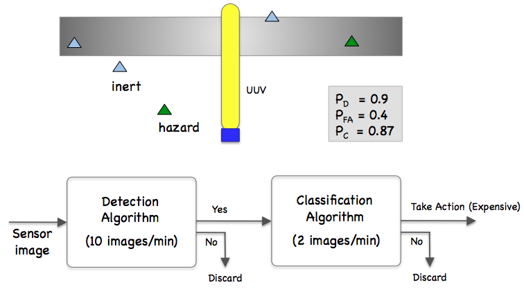
Figure 1.1: Simulated Hazard Sensor: A vehicle processes a series of sensor images which may or may not contain an object. The detection algorithm processes the image and rejects images it believes does not contain contain hazardous objects. It passes on images containing possible hazardous objects to a classifier, which makes a determination for each object in an incoming image as to whether or not the object is hazardous or benign.
In the uFldHazardSensor application, the objects and their properties (position, type, etc.) are read from a pre-generated hazard file.
The vehicle locations are known to the simulator from node reports received from the vehicles. And sensor output is sent to the vehicle in tidy UHZ_DETECTION_REPORT and UHZ_HAZARD_REPORT messages as a proxy to the actual hazard sensor and the calculations that would otherwise reside on the vehicle. The simulated sensor is configured to have a finite list of sensor settings, each consisting of a swath width, ROC curve, and probability of correct classification. It's up to the user to choose the sensor setting and choose a PD on the associated ROC curve, which determines the prevailing PFA.
2 A Quick Start Guide to Using uFldHazardSensor
To get started, we (a) point you to an example mission using uFldHazardSensor, (b) lay out the absolute minimum uFldHazardSensor configuration components, i.e., those which do not have default values, and (c) discuss the structure of a simple hazard file representing the ground-truth set of objects used by the simulated sensor.
2.1 A Working Example Mission - the Jake Mission [top]
The example mission is referred to as the Jake example mission and may be found and launched in the moos-ivp distribution with:
  $ cd moos-ivp/ivp/missions/m10_jake
  $ ./launch.sh 12
This launches the simulation with time warp 12. The time warp may be adjusted to suit your preference and is bounded above by your computer's processing capability. After launching and hitting the deploy button, you should see something similar to Figure 2.1.
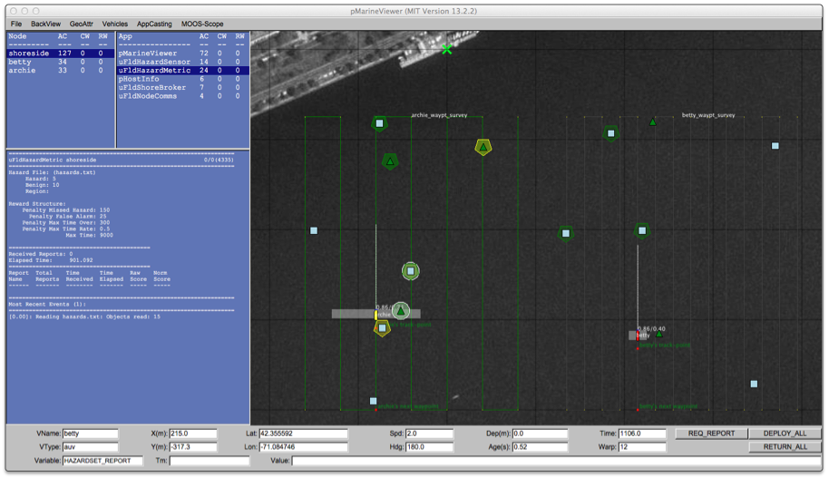
Figure 2.1: The Jake Example Mission: The jake example mission is involves a two vehicles each using the hazard sensor, traversing a search area using a lawnmower pattern. Both vehicles process their information and generate a hazardset report when finished.
There are few notable components of this simulation that comprise the hazard search nature of the mission:
- uFldHazardSensor: The simulated sensor itself.
- uFldHazardMetric: A MOOS app running on the shoreside that will grade the incoming hazardset reports generated by the vehicle. This is described in the uFldHazardMetric documentation.
- hazards.txt: A text file representing the ground truth laydown of objects in the search area. (Section 5.2).
- uFldHazardMgr: A straw-man MOOS app running on each vehicle to request sensor information, process the information, and generate a hazardset report upon request or the end of the mission.
2.2 A Bare-Bones Example uFldHazardSensor Configuration [top]
Listing 2.1 below shows a bare-bones configuration. Line 3 names a hazard file, containing the ground truth description of objects in the field. This format is described in Section 5, and an example hazard file is in the same directory as the Jake example mission.
Listing 2.1 - Example bare-bones configuration of uFldHazardSensor.
[[#lst_ufhz_bare_econfig]]
  1  ProcessConfig = uFldHazardSensor
  2  {
  3    hazard_file   = hazards.txt
  4
  5    sensor_config = width=25, exp=4, pclass=0.80
  6    sensor_config = width=50, exp=2, pclass=0.60
  7    sensor_config = width=10, exp=6, pclass=0.93
  8  }
The possible sensor configuration options are listed in lines 5-7. These values are from the Jake example mission and perhaps are reasonable values for any mission, but they are not the default. These options, a hazard_file and at least one sensor_config option, must be specified or the sensor will not operate. The sensor_config parameter is discussed in Section 4.2. The full set of configuration parameters for uFldHazardSensor is provided in Section 10, along with an extended example configuration file.
2.3 A Simple Hazard File [top]
In the Jake example mission, search is performed over a region containing a number of objects, some hazards, and some benign. The type and location of objects is defined in a hazard file. The hazard file for the Jake mission is shown below, and contains a single line for each object. The first line in the file is a copy of the command-line invocation used in generating this file. This command-line tool, gen_hazards is discussed in Section 5.2. An object in the file is comprised minimally of four components:
- The x location of the object,
- The y location of the object,
- The label of the object, unique across all objects,
- The type of the object.
 // gen_hazards --polygon=-150,-75:-150,-400:400,-400:400,-75 --objects=5,hazard --objects=10,benign
 hazard = x=-52,y=-290,label=75,type=hazard
 hazard = x=41,y=-108,label=53,type=hazard
 hazard = x=-64,y=-124,label=98,type=hazard
 hazard = x=232,y=-80,label=91,type=hazard
 hazard = x=239,y=-315,label=19,type=hazard
 hazard = x=-41,y=-246,label=82,type=benign
 hazard = x=185,y=-93,label=64,type=benign
 hazard = x=-150,y=-201,label=11,type=benign
 hazard = x=-76,y=-82,label=14,type=benign
 hazard = x=-73,y=-309,label=28,type=benign
 hazard = x=346,y=-371,label=73,type=benign
 hazard = x=-83,y=-390,label=77,type=benign
 hazard = x=220,y=-201,label=15,type=benign
 hazard = x=134,y=-204,label=95,type=benign
 hazard = x=370,y=-107,label=99,type=benign
Each object may contain additional components discussed in later sections.
2.4 Typical Simulator Topology [top]
The typical module topology is shown in Figure 2.2 below. Multiple vehicles may be deployed in the field, each periodically communicating with a shoreside MOOS community running a single instance of uFldHazardSensor. Each vehicle regularly sends a node report to the shoreside community read by uFldHazardSensor. The hazard sensor also is launched with a file indicating the actual simulated hazard field, with each object having a location, classification and label. In short the hazard sensor knows ground truth, the location and orientation of all vehicles and the sensor settings for all vehicles.
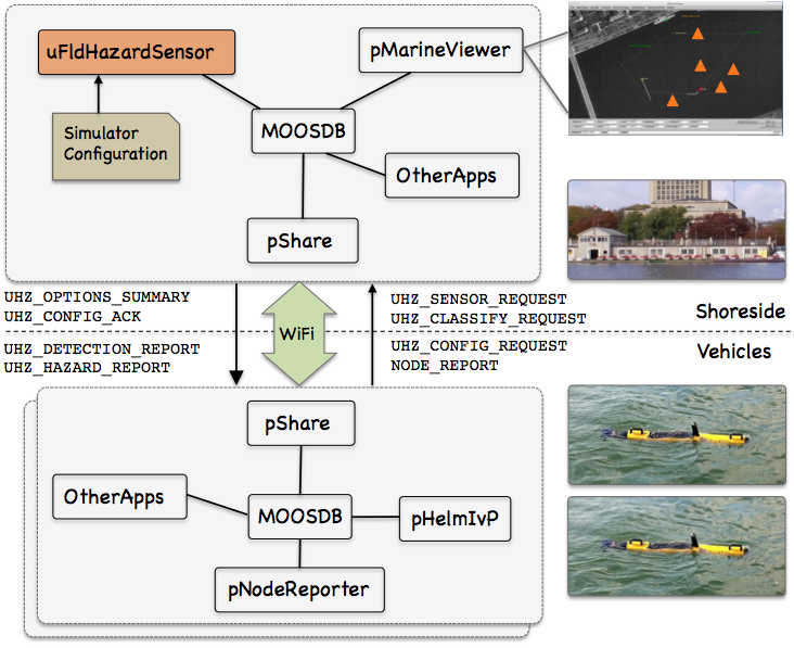
Figure 2.2: Typical uFldHazardSensor Topology: The simulator runs in a shoreside computer MOOS community and is configured with a hazard field containing both hazardous and benign objects. Vehicles accessing the simulator send a steady stream of messages (UHZ_SENSOR_REQUEST) and node reports to the shoreside community. The simulator continuously checks the connected vehicle's position against objects in the hazard field, and the sensor settings. When/if an object comes into sensor range, the simulator rolls the dice and if a detection is made, will send a UHZ_DETECTION_REPORT message to the vehicle. The vehicle may periodically re-configure its sensor setting by posting to UHZ_CONFIG_REQUEST. If the configuration request is acceptable, the simulator will respond with a message to UHZ_CONFIG_ACK bridged back out to the vehicle.
A vehicle operates its sensor by sending a steady stream of messages to the sensor on the shoreside under the variable UHZ_SENSOR_REQUEST. Each time the simulator receives this request, it will assess the vehicle's current position, and sensor settings, and may (depending on how the dice are rolled and if a detection is made) post a UHZ_DETECTION_REPORT to be bridged back out to the given vehicle. If the sensor does not make a detection, no report is sent.
Once the vehicle has made a detection, it may then make a further request of the hazard sensor to apply the classification algorithm to the given detection, by posting to variable UHZ_CLASSIFY_REQUEST, which also is bridged to the shoreside and handled by the hazard sensor. Regardless of the outcome, the hazard sensor will post a report, UHZ_HAZARD_REPORT indicating whether the detected object was either a hazard or a benign object. The frequency in which classification requests are handled is limited, by default to once per 30 seconds, but may be changed by setting the min_classify_interval parameter in the uFldHazardSensor configuration.
If running a pure simulation (no deployed vehicles), both MOOS communities may simply be running on the same machine configured with distinct ports. The pShare application is shown here for communication between MOOS communities, but there are other alternatives for inter-community communication and the operation of uFldHazardSensor is not dependent on the manner of inter-communication communications.
3 Detections and Classifications
Each time a vehicle passes over an object in the field, with the object entering the vehicle's sensor swath and exiting again, we refer to this as a sensor event, depicted in Figure 3.1. Although the simulated sensor does not deal with sensor images, the actions of the sensor simulator after each event may be thought as dealing with a hypothetical sensor image of the object gathered while it was in the sensor swath.
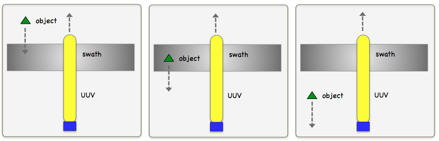
Figure 3.1: A Sensor Event: An sensor event occurs when an object enters the sensor swath. Following events for the same object may occur later after the object has exited the sensor swath.
For each sensor event, the simulator may generate two reports, a detection report and a classification report. The first is generated and returned to the vehicle unsolicited, while the latter is generated by the simulator only if the vehicle requests a classification report. The likelihood of a detection report and the likelihood of a correct classification are dependent on (a) the sensor settings, (b) the properties of the object being sensed, and (c) the relative angle of the vehicle sensor swath as is passes over the object.
3.1 The Simulated Detection Algorithm [top]
The sensor simulator handles multiple vehicles and multiple vehicle sensor setting choices. For each vehicle, the simulator is receiving node reports (NODE_REPORT), allowing the simulator to know each vehicle's present position. Of course the simulator also knows the hazard field configuration. Armed with these three pieces of information, (a) the sensor setting, (b) the vehicle position, and (c) the hazard field, it repeatedly operates in the manner shown in Figure 3.2 below.
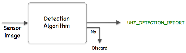
Figure 3.2: The simulated detection algorithm: Each time an object comes into the sensor field, it is considered once for detection. Once it goes out of the field, it may be processed again later if it comes back into the sensor field. If it passes the detection threshold, a detection report is posted to the MOOSDB. Otherwise no action is taken.
Each time an object comes into the sensor field for a vehicle, the simulator makes a detection determination based on:
- If the object is a hazard (ground-truth identified as such in the hazard configuration file), the simulator will report a detection with probability PD.
- If the object is benign the simulator will report a detection with probability PFA.
Again, the sensor swath width and PD are chosen by the vehicle, and PFA is set based on the chosen PD and sensor characteristics. This is discussed in detail in Section 4. If no detection is made, no further communication or action is taken by the simulator. If a detection is declared, a report is generated by the simulator to be shared to the vehicle:
UHZ_DETECTION_REPORT_ARCHIE = x=51,y=11.3,label=12
Note this report contains the object's unique identifier which relieves the user of the problem of data association.
3.2 The Simulated Classification Algorithm [top]
Once a detection has been made for an object, the object may be processed by the simulated classification algorithm. The idea is that the same set of raw sensor data, or image, is first passed through a quick detection filter, and the images for selected detections are then passed through a second, more resource-intensive, classification filter. This process may also be thought of as a proxy for offloading images through acoustic communications to another platform for processing. Either way, the idea is that the detection algorithm is fast, able to handle all raw data as is comes in, and the classification algorithm is more accurate but slower, forcing the careful consideration of which images to process.
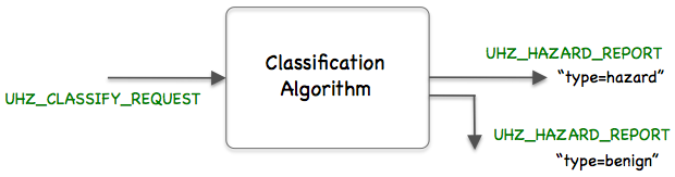
Figure 3.3: Simulated classification algorithm: The data from a given detection is processed by a separate algorithm for classifying the object as either a hazard or benign.
A classification request is made by the vehicle with a posting similar to the following:
UHZ_CLASSIFY_REQUEST = vname=archie,label=152
This variable would published by the vehicle, named archie, and would be shared to the shoreside community. The requesting vehicle knows the label value presumably from a prior received detection report. For each classification request received by uFldHazardSensor, the simulator makes a classification determination based the ground-truth declared in the hazard file, and the value of PC:
- If the object is a hazard, the simulator will report it as a hazard with probability PC.
- If the object is benign the simulator will report it as benign with probability PC.
Again, the value of PC is tied to the prevailing sensor setting chosen for that vehicle. After the classification determination has been made, a report is generated by the simulator to be shared to the vehicle:
UHZ_HAZARD_REPORT_ARCHIE = label=12,type=benign
Limiting the Classification Query Interval [top]
A limit is imposed by uFldHazardSensor on the frequency in which classification requests are processed. The default is one classification per 30 seconds. This may be configured differently with the min_classify_interval configuration parameter.
A classification request will be honored by uFldHazardSensor at any time after a detection has been made. Subsequent requests will be honored for each new pass over the object. In other words, uFldHazardSensor will not honor multiple classification request for a single pass over the object.
Managing the Order of Classification Requests [top]
By default, the classify requests are handled in the order in which they are received. This may be overridden to accommodate further consideration of the value of the classification information. The vehicle may associate a priority with the classify request, with a posting such as:
UHZ_CLASSIFY_REQUEST = vname=archie,label=152,priority=95
It is up to the user to determine the appropriate priority, perhaps tying the priority to the expected information gain. The user may also make a request that simply must be the top priority upon arrival. This can be done with a posting such as:
UHZ_CLASSIFY_REQUEST = vname=archie,label=152,priority=100,action=top
The above request will ensure that object 152 will be processed next. Each time a new entry is pushed into the top of the priority queue in this manner, the clock is reset for that vehicle, and min_classify_interval seconds will need to elapse before the next classify result is posted for that vehicle. The FIFO ordering is only relevant for two requests of equal priority, and all requests have a priority of 50 if the priority is left unspecified. One further tool available to the user is to simply clear the queue of pending requests completely:
UHZ_SENSOR_CLEAR = vname=archie
4 Simulator Sensor Configuration Options
The uFldHazardSensor simulator needs to be configured with one or more sensor settings. A sensor setting is comprised of the following 3-tuple:
- Swath width
- ROC curve exponent
- Classifier constant
These tuples are set in the uFldHazardSensor configuration block, and may then be chosen dynamically by the autonomy system on the vehicle by posting to the MOOS variable UHZ_CONFIG_REQUEST, by simply naming the requested swath width, and desired probability of detection. By default the hazard sensor limits the frequency of changes to the swath width setting. The default is 300 seconds. This is determined in the uFldHazardSensor configuration block with the parameter min_reset_interval. The probability of detection,  , may be changed as often as desired.
4.1 Sensor Swath Width Options [top]
The sensor swath width specifies the width of the sensor field at any given moment, from center of the vehicle out to either the port or starboard side. The swath length is set in the uFldHazardSensor configuration block and remains the same regardless of the swath width.
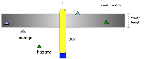
Figure 4.1: Sensor Swath Parameter: The swath width is a parameter that may be re-configured dynamically by the autonomy system. The swath length is set once in the uFldHazardSensor configuration block.
4.2 Sensor ROC Curve Configuration Options [top]
The ROC curves used in this simulator are based on a simple relationship between probability of detection, PD, and probability of false alarm, PFA. An example ROC curve is shown in 4.2. This curve represents

The user of a given sensor with this characteristic ROC curve must decide where to set the detection threshold, PD. By selection a higher PD, one must also have to live with a higher PFA. Since the user usually approaches this problem by choosing the PD, the curve in the figure below could also be described as:

The PFA typically follows from a user-chosen PD. For this reason, the uFldHazardSensor simulator is configured by identifying the ROC curve solely by the exponent value in the above function.
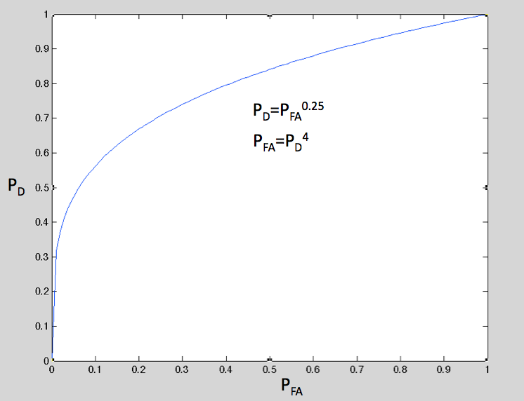
Figure 4.2: Example Receiver Operating Characteristic (ROC) Curve: The ROC curve relates the probability of detection, PD, on the y-axis, vs. the probability of false alarm, PFA, on the x-axis.
The above ROC may correspond to, for example, the below sensor configuration in the uFldHazardSensor configuration block:
sensor_config = width=25, exp=4, pclass=0.80
The sensor may be configured with more than one ROC curve, typically trading off a more desirable ROC curve for a small sensor swath. For example, the simulated sensor may be configured with the following five options:
  sensor_config = width=80, exp=2, pclass=0.60
  sensor_config = width=65, exp=4, pclass=0.75
  sensor_config = width=50, exp=6, pclass=0.85
  sensor_config = width=30, exp=12, pclass=0.93
  sensor_config = width=18, exp=20, pclass=0.97
The idea is shown in Figure 4.3. When the sensor is configured with these options, it presents the user with two choices to make: the sensor width, and choice for PD. This is done with the UHZ_CONFIG_REQUEST interface described in Section 4.4.
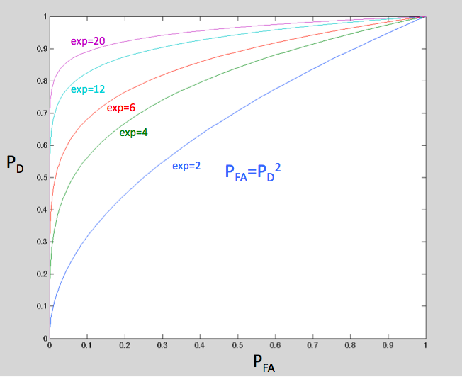
Figure 4.3: Example ROC Curve Configuration Options: By altering a single component, the exponent component of the expression  , the ROC curve characteristics may be varied from least desirable (exp=1) to most desirable (exp=20 or higher).
If the sensor user (a given vehicle) does not request a particular swath width and PD, the simulator will choose one of the options as a default. The default swath width is selected by choosing the highest width that is not more than the average between the highest and lowest width. In the settings above, for example, the width=30 is the highest width not greater than the average of the two extremes (49). The default PD setting is 0.9 if left unspecified.
4.3 Classification Configuration Options [top]
Classification refers to the process of handling a detected object and determining if it is either a hazard or a benign object (false alarm), described in Section 3.2. The classification stage is shown in Figure 1.1. In the simulator, this is simply implemented by rolling the dice according to a single probability metric PC. This is the probability that the classification determination is correct. Since PC=1 and PC=0 provide the same net utility, the range of values for PC is from [0.5,1]. This value is tied to a particular swath width and ROC curve characteristic. The idea is that a smaller swath width allows the sensor to provide a denser set of image data for a smaller area, which leads to both the better ROC curve as well as crisper images for a classification algorithm (even if the classifying agent is a human examining images off-board).
4.4 Dynamic Resetting of the Sensor [top]
The uFldHazardSensor simulator is configured with a set of configuration options, as described above, of which one must be chosen, along with a chosen PD. This is done by the vehicle posting a configuration request of the form:
UHZ_CONFIG_REQUEST = vname=archie, width=32, pd=0.95
The first field tells the simulator which vehicle is making the request. The second field identifies the ROC curve and swath width. The last field identifies the point on the ROC curve and thus determines the PFA. The uFldHazardSensor simulator processes this request by matching up the request to the set of possible options. If the exact swath width requested is not available, the next lowest is chosen. If the requested swath width is less than the lowest option, the lowest option is chosen. The simulator sends an acknowledgment to the vehicle in the form of:
UHZ_CONFIG_ACK_ARCHIE = width=30,pd=0.9,pfa=0.28,pclass=0.93
The sharing of the variable UHZ_CONFIG_ACK_ARCHIE between the shoreside and the vehicle archie is handled by pShare, typically with dynamic registrations automatically configured by uFldShoreBroker. By default the hazard sensor limits the frequency of changes to the sensor settings. The default is 300 seconds. This is determined in the uFldHazardSensor configuration block with the parameter min_reset_interval. This only restricts how often the swath width may be reset. The desired value for the probability of detections, PD, may be reset as often as desired. In this case the configuration request would simply not specify a desired swath width. For example:
UHZ_CONFIG_REQUEST = vname=archie, pd=0.75
4.5 Posting of Sensor Configuration Options [top]
The sensor configuration options may be known to other MOOS processes by subscribing to the MOOS variable, UHZ_OPTIONS_SUMMARY. The following would be published:
  UHZ_OPTIONS_SUMMARY = width=25,exp=4,pclass=0.85:width=50,exp=2,pclass=0.60 [=\=]
                        width=10,exp=6,pclass=0.93
corresponding to the following configuration of uFldHazardSensor:
  sensor_config = width=25, exp=4, pclass=0.85
  sensor_config = width=50, exp=2, pclass=0.60
  sensor_config = width=10, exp=6, pclass=0.93
Since this information rarely if ever changes after its first posting, it is not posted very often. By default it is posted once every ten seconds. Since this posting is typically occurring on a shoreside computer, bridged to a remote vehicle, a long delay may not be desirable. This interval may be altered, for example to 5 seconds, by configuring options_summary_interval=5.
5 Configuring the Hazard Field
The hazard field is configured either by reading in a hazard file, or by explicitly listing the hazards in the uFldHazardSensor configuration block. The former method is recommended since the hazard file is typically also read by uFldHazardMetric for grading hazardset reports against the ground truth. The ground truth obviously needs to be the same between applications and this is easier to ensure if they are just pointing to the same file. Either way, the format for specifying an object is the same and has the following fields by example:
hazard = x=98.2,y=-127.7,label=14,type=benign
Below is a list of possible fields for specifying an object. The first for fields, used in the example above are mandatory. Uniqueness between labels is mandatory as well.
- [x] position
- [y] position
- [type] (hazard or benign)
- [label] (unique between entries)
An optional fields for specifying a hazard resemblance factor, discussed further in Section 6:
- [hr]: a value in the range [0,1] associated with benign objects
Optional fields for specifying an optimal aspect angle for correctly detecting and classifying an object, discussed further in Section 7:
- [aspect]: the optimal sensing aspect angle
- [aspect_min]: the aspect angle range within which sensing is still optimal
- [aspect_max]: the aspect angle range beyond which sensing is fully degraded
Optional fields for specifying rendering hints on a per-object basis:
- [color] (rendering hint, default: green for hazards, light_blue for benign objects)
- [shape] (rendering hint, default: triangle for both hazards and benign objects)
- [width] (rendering hint, default: 8 meters for both hazards and benign objects)
So an object specification utilizing all object parameters may look like:
  hazard = x=98.2,y=-127.7,label=14,type=benign,hr=0.8,aspect=43,aspect_min=30,
           aspect_max=60,color=yellow,shape=square,width=4
5.1 An Example Hazard Field [top]
The field in Figure 5.1 below shows an example field. This is also the hazard field used in the example mission, m10_jake, described briefly in Section 2.1, and more fully in Section 13.
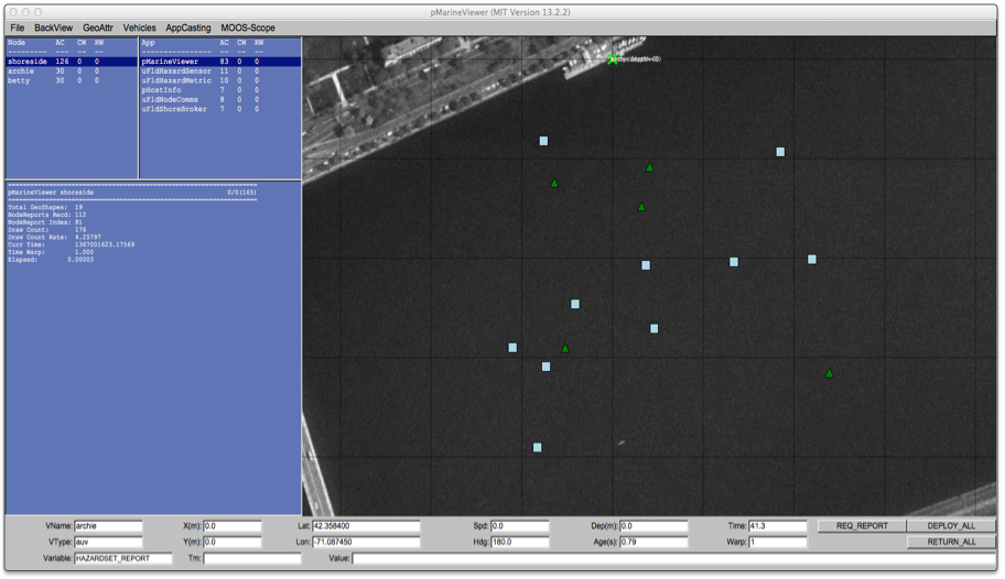
Figure 5.1: Simulated Hazard Field: A hazard field with 18 objects is shown, some are hazardous objects, some are benign objects.
The hazard field may be configured with either entries in the uFldHazardSensor configuration block, or by reading in a hazard field configuration file. The format for a configuration line is the same in both cases. For the hazard field shown in Figure 5.1, the configuration lines used were:
  hazard = x=-52,y=-290,label=75,type=hazard
  hazard = x=41,y=-108,label=53,type=hazard
  hazard = x=-64,y=-124,label=98,type=hazard
  hazard = x=32,y=-148,label=91,type=hazard
  hazard = x=239,y=-315,label=19,type=hazard
  hazard = x=-41,y=-246,label=82,type=benign
  hazard = x=185,y=-93,label=64,type=benign
  hazard = x=-110,y=-290,label=11,type=benign
  hazard = x=-76,y=-82,label=14,type=benign
  hazard = x=-73,y=-309,label=28,type=benign
  hazard = x=46,y=-271,label=73,type=benign
  hazard = x=-83,y=-390,label=77,type=benign
  hazard = x=220,y=-201,label=15,type=benign
  hazard = x=134,y=-204,label=95,type=benign
  hazard = x=37,y=-207,label=99,type=benign
5.2 Automatically Generating a Hazard Field [top]
There also exists in the moos-ivp tree a small utility call gen_hazards. This simple command line tool will generate a list of randomly generated objects of a specified type, given a convex polygon as input. For example:
  $ gen_hazards --polygon=-150,-75:-150,-400:400,-400:400,-75 --objects=5,hazard
    --objects=10,benign
  hazard = x=-52,y=-290,label=75,type=hazard
  hazard = x=41,y=-108,label=53,type=hazard
  hazard = x=-64,y=-124,label=98,type=hazard
  hazard = x=32,y=-148,label=91,type=hazard
  hazard = x=239,y=-315,label=19,type=hazard
  hazard = x=-41,y=-246,label=82,type=benign
  hazard = x=185,y=-93,label=64,type=benign
  hazard = x=-110,y=-290,label=11,type=benign
  hazard = x=-76,y=-82,label=14,type=benign
  hazard = x=-73,y=-309,label=28,type=benign
  hazard = x=46,y=-271,label=73,type=benign
  hazard = x=-83,y=-390,label=77,type=benign
  hazard = x=220,y=-201,label=15,type=benign
  hazard = x=134,y=-204,label=95,type=benign
  hazard = x=37,y=-207,label=99,type=benign
If the information is stored in file, then uFldHazardSensor may then be configured with the single line hazard_file=hazards.txt. This utility also supports command line options for randomly generating hazard resemblance factors and aspect information for each object.
6 Hazard Resemblance Factor
The simulator may be configured with benign objects that have an optional resemblance factor. This is a number in the range [0,1], where zero indicates the object looks absolutely nothing like a hazard, and one indicates a very close resemblance to a hazard. When this factor is present, it affects both the probability of detection, PD, and the probability of classification, PC. Such objects are configured like any other object, but have an additional parameter, for example:
hazard = x=37,y=-207,label=99,type=benign,hr=0.73
6.1 The Effect of the Resemblance Factor on Detections [top]
The general detection algorithm was described in Section 3.1. In short, hazards generate detections with probability PD, and benign objects (falsely) generate detections with probability PFA. When a benign object has a hazard resemblance factor, R, the probability of false alarm is instead (PFA + R) /2. Since the R factor has a range of [0,1], the modified probability also still has a range of [0,1].
6.2 The Effect of the Resemblance Factor on Classifications [top]
As with detections, the hazard resemblance factor only affects the probability of correct classifications for benign objects. If the object is benign and does have an associated hazard resemblance factor, R, the simulator will report it as benign with probability PC + (1 - PC)(1-R). In other words, if a benign object happens to have a very high resemblance to a hazard, R ~=1 , the probabibliy of a correct classification is at its lowest, PC. If the benign objects happens to have very little resemblence to a hazard, R ~= 0, the probability of classificatin is at its highest, nearly 1.
6.3 Generating a Random Hazard Field with Resemblance Factors [top]
A hazard resemblance factor may be automatically generated with the gen_hazards utility by including an optional command-line argument, --exp=N, where N is in the range [0.01,10]. When this argument is provided, the utility starts by generating, for each benign object, a resemblance factor over the range [0,1] with uniform probability. It then raises this value to the number provided by the --exp parameter. The higher this parameter, the lower the expected value for the resulting resemblance factors. For example, with --exp=1:
 gen_hazards --polygon=-150,-75:-150,-400:400,-400:400,-75 --objects=4,benign --exp=1
 hazard = x=149,y=-216,label=82,type=benign,hr=0.605
 hazard = x=263,y=-88,label=51,type=benign,hr=0.874
 hazard = x=292,y=-185,label=96,type=benign,hr=0.306
 hazard = x=-57,y=-194,label=91,type=benign,hr=0.07
 hazard = x=-144,y=-330,label=58,type=benign,hr=0.801
With --exp=10:
 gen_hazards --polygon=-150,-75:-150,-400:400,-400:400,-75 --objects=4,benign --exp=10
 hazard = x=390,y=-137,label=39,type=benign,hr=0.00001
 hazard = x=236,y=-213,label=46,type=benign,hr=0.12772
 hazard = x=172,y=-215,label=76,type=benign,hr=0.01033
 hazard = x=-114,y=-235,label=8,type=benign,hr=0.40688
With --exp=0.01:
 gen_hazards --polygon=-150,-75:-150,-400:400,-400:400,-75 --objects=4,benign --exp=0.01
 hazard = x=226,y=-379,label=85,type=benign,hr=0.96231
 hazard = x=231,y=-167,label=81,type=benign,hr=0.92962
 hazard = x=108,y=-101,label=74,type=benign,hr=0.78424
 hazard = x=225,y=-379,label=86,type=benign,hr=0.9767
6.4 Disabling the Hazard Resemblance Factor [top]
The hazard resemblance factors can be effectively disabled by configuring uFldHazardSensor with ignore_resemblances=true. The default is false.
7 Aspect Angle Sensitivity
The simulator may be configured with objects having an aspect sensitivity. In this case, a unique optimal aspect angle may be associated with each object. Depending on the vehicle's approach angle to the object, the sensor performance may be degraded the further the approach angle deviates from the optimal aspect angle. Such objects are configured like any other object, but have three additional parameters, for example:
hazard = x=37,y=-207,label=99,type=benign,aspect=57,aspect_min=20,aspect_max=45
The idea is that the vehicle heading, as its sensors pass over the object, is relevant to the sensor performance. If the vehicle heading matches the object's optimal aspect angle, the sensor data collected is optimal with respect to the simulated sensor processing algorithms. The more the vehicle approach heading differs from the optimal aspecte angle, the more the sensor is degraded in terms of PD, PFA, and PC.
To be more precise, a sensor degradation value is calculated, in the range of [0, 1], i.e., zero to one hundred percent. This value is determined by first calculating the heading_delta, representing difference in vehicle approach heading compared to the object's optimal aspect angle. This value is in the range [0,90], with zero meaning the vehicle approach heading was dead-on perfect with the object's optimal aspect angle. The simulator knows the vehicle_heading from incoming node reports, and the optimal aspect angle, aspect, aspect_min, and aspect_max for an object based on the ground truth hazard file. First, the heading_delta is determined by:

Then, the sensor degradation is determined by:

The degradation value is used to the modify the detection and classification algorithms, described next.
7.1 The Effect of Aspect Sensitivity on the Detection Algorithm [top]
The general detection algorithm was described in Section 3.1. In short, hazards generate detections with probability PD, and benign objects (falsely) generate detections with probability PFA. The relationship between PD and PFA is based on the ROC curve associated with the prevailing sensor settings. Aspect sensitivity is applied in a two step process:
- Determination of sensor degradation as described above, and
- Application of sensor degradation based on a modified ROC curve.
A full (one hundred percent) sensor degradation essentially is equivalent to the sensor working with a ROC curve of exponent 1, a linear line, as discussed in Section 4.2, and in Figure 4.2. In this case, PD and PFA are equivalent at all points on the curve; a detection event provides no insight into the object type. When there is no sensor degradation, the form of the ROC curve remains unchanged. In between, with partial sensor degradation, the ROC curve is somewhere in between its original form and 1 (linear). For example, if the original ROC curve was formed with an exponent of 5, 50% sensor degradation entails a ROC curve of 3 instead. If the user had chosen a PD of 0.9, the corresponding PFA would have been  but is instead
  with 50% degradation.
7.2 The Effect of Aspect Sensitivity on the Classification Algorithm [top]
The general classification algorithm was described in Section 3.2. In short, each time a classification request is processed, the probability of a correct classification is PC. This holds whether the actual object is a hazard or benign object. Aspect sensitivity is applied in a two step process:
- Determination of sensor degradation as described above, and
- Application of sensor degradation to modify the probability of classification to this object on this pass.
A full sensor degradation is equivalent to setting PC=0.5, which is essentially as good as a random coin flip. For partial degradations, the PC is revised downward:

7.3 Visual Cues on Aspect Sensitivity [top]
Normally uFldHazardSensor generates visual cues upon detections and classifications; white circles on a detection, yellow or green pentagons upon classification reports. To aid things further, the application calculates detection and classification results with and without aspect sensitivity. When the sensor degradation is noted to have an adverse effect, the interior of the circles or polygons are filled in with a pink color rather than their normal white, green or yellow color.
7.4 Configuring the Simulator Visual Preferences [top]
As shown in Figure 2.2, the uFldHazardSensor is typically running in the shoreside community, alongside a GUI application like pMarineViewer. Certain messages are posted by uFldHazardSensor for visualization by default. They may be shut off, or have their properties altered by configuring the simulator as desired.
7.5 Configuring the Sensor Field Swath Rendering [top]
The sensor field is normally rendered as a rectangle that moves along with the vehicle. This rectangle is drawn to exactly correspond to the sensor field. Rendering in pMarineViewer is accomplished by a posting of VIEW_POLYGON by uFldHazardSensor. This may be shut off with the following configuration:
show_swath = false
The swath is slightly transparent to allow for the objects to be seen under the swath. The default transparency is 0.2, but may be changed with the following configuration:
swath_transparency = 0.60
While the length of the rendered swath width from side to side is determined by the sensor setting, the length of the rendered swath width from front to back is determined by the configuration:
swath_length = 5 // In meters. 5 is the default.
7.6 Configuring the Hazard Field Renderings [top]
Rendering of the hazard field is done at the start of uFldHazardSensor by producing a VIEW_MARKER posting once for each object in the field. This may be disabled with:
show_hazards = false
Although each object in the hazard file may be configured with color, shape, and width, the default values may be provided for any object that leaves any one of these fields unspecified.
  default_hazard_shape = triangle
  default_hazard_color = green
  default_hazard_width = 8
  default_benign_shape = triangle
  default_benign_color = green
  default_benign_width = 8
7.7 Configuring the Sensor Report Renderings [top]
Sensor reports are rendered as circles around the objects in the hazard field. If a detection is not made, no circle is rendered. If a detection is made and classified as a hazard, a yellow pentagon is rendered. If classified as benign, a green pentagon is rendered. All such renderings are accomplished by uFldHazardSensor making a posting to VIEW_CIRCLE, then processed by pMarineViewer.
When multiple vehicles are using the simulator, it may be confusing after some time to know which vehicle was responsible for which object rendered. For this reason, the uFldHazardSensor may be configured to have the detection circles disappear after some number of seconds. This can be done with:
show_detections = 60
The above will result in each detection circle being rendered for 60 seconds before disappearing from view.
7.8 Rendering the Prevailing PD and PFA Values [top]
Normally the prevailing PD and PFA values are rendered alongside the vehicle's sensor swath as shown in Figure 7.1. These may be either configured on or off with the following two configuration parameters:
  show_pd  = true  // the default is true
  show_pfa = true  // the default is false
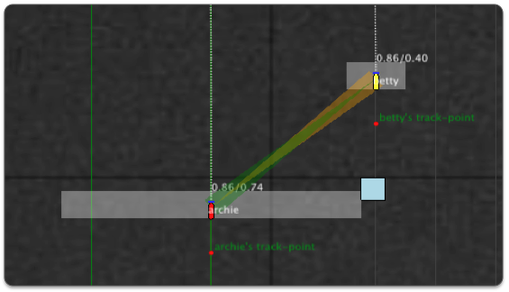
Figure 7.1: The prevailing PD and PFA values may be optionally rendered alongside the sensor swath.
8 Under the Hood: Sensor Blackouts During Turns
Image data collected during turns is notoriously poor, effectively rendering that data useless for automatic image processing algorithms. The hazard simulator therefore has provisions to disable itself during turns. It does so by storing a recent vehicle heading history from node reports, and disabling detections during turns. The visual aspects of the sensor swath also change as shown in Figure 8.1.
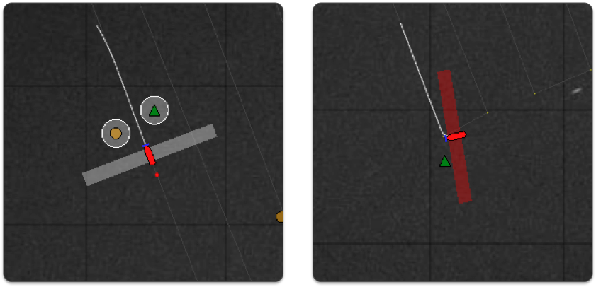
Figure 8.1: Sensor blackouts during turns: A vehicle will render its swath in white when running straight and on, and will render the swath in red when turning and disabled. In the image on the right, the vehicle may not have detected the object it just passed even if it were not turning, but in this case the lack of detection was ensured due to the turning of the vehicle.
By default the sensor will be disabled when the recent turn rate (defined over the previous 2 seconds) exceeds a rate of 1.5 degrees per second. This may be adjusted in the mission file with the following parameter:
max_turn_rate = 3.0
9 Under the Hood: Maximum Vehicle Speed
The simulator by default will enforce a maximum vehicle speed above which no reliable sensor data will be obtainable. This maximum speed is 2.0 meters per second by default and may be changed with the configuration parameter:
max_vehicle_speed = 3.0
10 Configuration Parameters of uFldHazardSensor
The following parameters are defined for uFldHazardSensor. A more detailed description is provided in other parts of this section. Parameters having default values are indicated so.
Listing 10.1 - Configuration Parameters for uFldHazardSensor.
| default_benign_color: | Color for rendering benign objects. Legal values: any color in Color Appendix. The default is lightblue. Section 7.6. |
| default_benign_shape: | Shape for rendering benign objects Legal values: square, circle, diamond, triangle. The default is triangle. Section 7.6. |
| default_benign_width: | Width in meters for rendering benign objects. The default is 8. Section 7.6. |
| default_hazard_color: | Color for rendering hazard objects. Legal values: any color in the Color Appendix. The default is green. Section 7.6. |
| default_hazard_shape: | Shape for rendering hazard objects. Legal values: square, circle, diamond, triangle. The default is triangle. Section 7.6. |
| default_hazard_width: | Width in meters for rendering hazard objects. The default is 8. Section 7.6. |
| hazard_file: | Names a file containing the hazard field configuration. Section 5. |
| ignore_resemblances: | If true, ignore any hazard resemblance factor associated with a hazard. Section 6.4. |
| max_turn_rate: | Maximum rate of turn in meters per second, above which the sensor will not produce detections. The default is 1.5. Section 8. |
| max_vehicle_speed: | Maximum vehicle speed in meters per second, above which the sensor will not produce detections. The default is 2.0. Section 8. |
| min_classify_interval: | Minimum amount of time between classification results per vehicle. The default is 30 seconds. Section 3.2. |
| min_reset_interval: | Minimum amount of time between sensor configuration resets per given vehicle. The default is 300 seconds. Section 4. |
| options_summary_interval: | Duration (secs) between posting of options summary. The default is 10. Section 4.5. |
| seed_random: | If true, a random number generated is seeded. Legal values: true, false. The default is true. |
| sensor_config: | Describes one of possibly many sensor config options. Section 4. |
| show_detections: | Duration attached to detection circle postings. Legal values: any numerical value or the keyword "nolimit". The default is nolimit. Section 7.7. |
| show_hazards: | If false, hazard field visuals are not posted. Legal values: true, false. The default is true. Section 7.6. |
| show_pd: | If true, the probability of detection, PD, associated with a particular vehicle will be rendered alongside the swath rendering. Legal values: true, false. The default is true. Section 7.8. |
| show_pfa: | If true, the probability of false alarm, PFA, associated with a particular vehicle will be rendered alongside the swath rendering. Legal values: true, false. The default is false. Section 7.8. |
| show_swath: | If false, vehicle sensor swath visuals are not posted. Legal values: true, false. The default is true. Section 7.5. |
| swath_transparency: | Transparency used for rendering swath. Legal values: [0,1]. The default is 0.2. Section 7.5. |
| swath_length: | Extent of the sensor swath, in meters, in the direction of bow to stern. Legal values: any numerical value. Values less than 1 will be clipped to 1. The default is 5. |
10.1 An Example MOOS Configuration Block [top]
To see an example MOOS configuration block, enter the following from the command-line:
$ uFldHazardSensor --example or -e
This will show the output shown in Listing 10.2 below.
Listing 10.2 - Example configuration for uFldHazardSensor.
[[#lst_ufhz_econfig]]
   1  ===============================================================
   2  uFldHazardSensor Example MOOS Configuration
   3  ===============================================================
   4
   5  ProcessConfig = uFldHazardSensor
   6  {
   7    AppTick   = 4
   8    CommsTick = 4
   9
  10    // Configuring visual preferences
  11    default_hazard_shape = triangle                 // default
  12    default_hazard_color = green                    // default
  13    default_hazard_width = 8                        // default
  14
  15    default_benign_shape = triangle                 // default
  16    default_benign_color = light_blue               // default
  17    default_benign_width = 8                        // default
  18    swath_transparency   = 0.2                      // default
  19
  20    sensor_config = width=25, exp=4, class=0.80
  21    sensor_config = width=50, exp=2, class=0.60
  22    sensor_config = width=10, exp=6, class=0.93,max=1
  23    hazard_file   = hazards.txt
  24    swath_length  = 5                               // default
  25    seed_random   = false                           // default
  26
  27    show_hazards  = true  // default                // default
  28    show_swath    = true  // default                // default
  29    show_detections = 60  // seconds (unlimited if unspecified)
  30    show_pd       = true  // pd shown with swaths   // default
  31    show_pfa      = true  // pfa shown with swaths  // default
  32
  33    min_reset_interval       = 300  // default
  34    min_classify_interval    = 30   // default
  35    options_summary_interval = 10   // default
  36  }
11 Publications and Subscriptions for uFldHazardSensor
The interface for uFldHazardSensor, in terms of publications and subscriptions, is described below. This same information may also be obtained from the terminal with:
$ uFldHazardSensor --interface or -i
11.1 Variables Published by uFldHazardSensor [top]
The primary output of uFldHazardSensor to the MOOSDB is posting of sensor reports, visual cues for the sensor reports, and visual cues for the hazard objects themselves.
- APPCAST: Contains an appcast report identical to the terminal output. Appcasts are posted only after an appcast request is received from an appcast viewing utility. Section 12
- UHZ_DETECTION_REPORT: A report on a detection made by the sensor for an object in the hazard field. It includes the name of the vehicle.
- UHZ_DETECTION_REPORT_NAMEJ: A report on a detection made by the sensor (on vehicle NAMEJ) for an object in the hazard field.
- UHZ_HAZARD_REPORT: A report on a classification made by the sensor for an object in the hazard field. It includes the name of the vehicle.
- UHZ_HAZARD_REPORT_NAMEJ: A report on a classification made by the sensor (on vehicle NAMEJ) for an object in the hazard field.
- UHZ_OPTIONS_SUMMARY: A report the possible sensor settings available to the user.
- UHZ_CONFIG_ACK: An acknowledgment message sent to the vehicle verifying a requested sensor setting.
- VIEW_CIRCLE: A visual artifact for rendering a circle around a hazard, indicating the detection and classification.
- VIEW_MARKER: A visual artifact for rendering objects in the hazard field.
- VIEW_POLYGON: A visual artifact for rendering a rectangle around a vehicle, indicating a vehicle sensor field moving with the vehicle.
Example postings:
  UHZ_DETECTION_REPORT        = vname=archie,x=51,y=11.3,label=12
  UHZ_DETECTION_REPORT_ARCHIE = x=51,y=11.3,label=12
  UHZ_HAZARD_REPORT           = vname=archie,x=51,y=11.3,hazard=true,label=12
  UHZ_HAZARD_REPORT_ARCHIE    = x=51,y=11.3,hazard=true,label=12
  UHZ_CONFIG_ACK              = vname=archie,width=20,pd=0.9,pfa=0.53,pclass=0.91
  UHZ_OPTIONS_SUMMARY         = width=10,exp=6,pclass=0.9:width=25,exp=4,pclass=0.85
The vehicle name may be embedded in the MOOS variable name to facilitate distribution of report messages to the appropriate vehicle with pShare.
11.2 Variables Subscribed for by uFldHazardSensor [top]
The uFldHazardSensor application will subscribe for the following MOOS variables:
- APPCAST_REQ: A request to generate and post a new apppcast report, with reporting criteria, and expiration.
- UHZ_CONFIG_REQUEST: A message from the vehicle requesting one of the possible sensor settings and PD choice from the ROC curve resulting from the sensor settings. See Section 4.4.
- UHZ_CLASSIFY_REQUEST: A message from the vehicle requesting a classification result for a given object. See Section 3.2.
- UHZ_SENSOR_REQUEST: A message from the vehicle indicating the sensor is active.
- NODE_REPORT: A report on a vehicle location and status.
Example postings
  UHZ_SENSOR_REQUEST = vname=archie
  UHZ_CONFIG_REQUEST = vname=archie,width=50,pd=0.9
Command Line Usage of uFldHazardSensor [top]
The uFldHazardSensor application is typically launched as a part of a batch of processes by pAntler, but may also be launched from the command line by the user. To see command-line options enter the following from the command-line:
$ uFldHazardSensor --help or -h
This will show the output shown in Listing 11.1 below.
Listing 11.1 - Command line usage for the uFldHazardSensor tool.
[[#lst_ufhz_usage]]
   1  ==========================================================
   2  Usage: uFldHazardSensor file.moos [OPTIONS]
   3  ==========================================================
   4
   5  Options:
   6    --alias=<ProcessName>
   7        Launch uFldHazardSensor with the given process
   8        name rather than uFldHazardSensor.
   9    --example, -e
  10        Display example MOOS configuration block.
  11    --help, -h
  12        Display this help message.
  13    --interface, -i
  14        Display MOOS publications and subscriptions.
  15    --version,-v
  16        Display release version of uFldHazardSensor.
  17    --verbose=<setting>
  18        Set verbosity. true or false (default)
  19
  20  Note: If argv[2] does not otherwise match a known option,
  21        then it will be interpreted as a run alias. This is
  22        to support pAntler launching conventions.
12 Terminal and AppCast Output
The uFldHazardSensor application produces some useful information to the terminal and identical content through appcasting. An example is shown in Listing 12.1 below. On line 2, the name of the local community, typically the shoreside community, is listed on the left. On the right, "0/0(457) indicates there are no configuration or run warnings, and the current iteration of uFldHazardSensor is 457. Lines 4-6 show the name of the ground truth hazard file and the number of hazards and benign objects.
Lines 8-16 convey the available sensor configuration options, set with the sensor_config parameter.
Listing 12.1 - Example uFldHazardSensor console output.
[[#lst_uhz_appcast]]
   1  ===================================================================
   2  uFldHazardSensor shoreside                                 0/0(457)
   3  ===================================================================
   4  Hazard File: (hazards.txt)
   5       Hazard: 11
   6       Benign: 8
   7
   8  ============================================
   9  Sensor Configuration Options
  10  ============================================
  11  Width  Exp  Classify
  12  -----  ---  --------
  13  10.0   6.0  0.930
  15  425.0   4.0  0.850
  16  50.0   2.0  0.600
  17
  18  ============================================
  19  Sensor Settings / Stats for known vehicles:
  20  ============================================
  21  Vehicle  Swath                        Sensor  Sensor
  22  Name     Width  Pd     Pfa    Pclass  Resets  Requests  Detects
  23  -------  -----  -----  -----  ------  ------  --------  -------
  24  archie   50.0   0.860  0.740  0.600   1(12)   203       0
  25
  26  ===================================================================
  27  Most Recent Events (1):
  28  ===================================================================
  29  [11.86]: Setting sensor settings for: archie
13 The Jake Example Mission Using uFldHazardSensor
The Jake mission is distributed with the MOOS-IvP source code and contains a ready example of the uFldHazardSensor application, configured with hazard field in an included text file. Assuming the reader has downloaded the source code available at www.moos-ivp.org and built the code according to the documentation, the Jake mission may be launched by:
  $ cd moos-ivp/ivp/missions/m10_jake/
  $ ./launch.sh 10
The argument, 10, in the line above will launch the simulation in 10x real time. Once this launches, the pMarineViewer GUI application should launch and the mission may be initiated by hitting the DEPLOY button.
13.1 What is Happening in the Jake Mission [top]
The Jake mission is comprised of two simulated vehicles, archie and betty. There are three MOOS communities launched, one for the shoreside and one each for the two vehicles. See Figure 2.2. The uFldHazardSensor simulator is running in the shoreside community. The Jake mission is comprised of two phases, the broad-area-search phase and the reacquire phase. In this mission, archie handles the first phase, passes his results to betty, who handles the second phase.
The Broad Area Search Phase [top]
In the broad-area-search phase, a search region is given to archie, in which it is to search for a set of objects, some of which may be hazardous. Knowing nothing a priori about the location of the objects, only the region containing them, archie executes a lawnmower search pattern over this area, as shown in Figure 13.1. The snapshot in the figure depicts archie having executed most of its pattern, to the West proceeding East. The hazard field is rendered with actual hazards drawn in green triangles, and benign objects drawn in light blue squares. The circles represent detections reported by uFldHazardSensor. The yellow circles represent objects classified as hazards, and the white circles represent objects classified as benign.
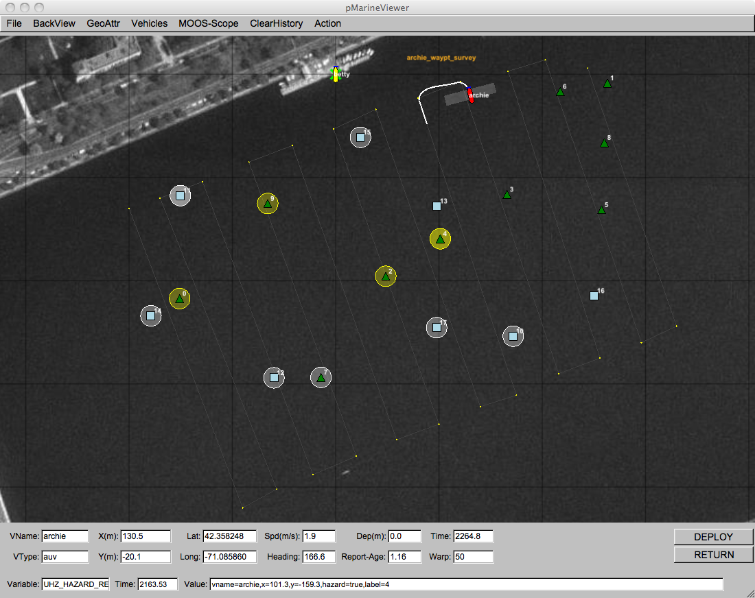
Figure 13.1: Simulated Hazard Sensor: A vehicle processes a series of sensor images which may or may not contain an object. The detection algorithm processes the image and rejects images it believes does not contain contain hazardous objects. It passes on images containing possible hazardous objects to a classifier, which makes a determination for each object in an incoming image as to whether or not the object is hazardous or benign.
In this mission, the vehicle's sensor is configured with a swath width of 25 meters (12.5 on either side), a probability of detection PD=0.9, probability of false alarm PFA=0.66, and probability of correct classification PC=0.85. Note in the above snapshot, the vehicle has successfully detected all hazards, but also detected all but one benign object. It has correctly classified all but one object.
The Reacquire Phase [top]
In the reacquire phase, the archie vehicle has returned to the dock, and betty vehicle has been a mission to revisit a set of points. In this case betty has an idea where those points lie and is following a simple path, as shown in Figure 13.2. Presumably the list of objects to visit and their locations have been communicated to betty from archie. (In this mission things were hard-coded, no message passing actually occurred.) The objective of betty is to use a sensor with a smaller swath width and better sensor processing algorithm to reduce the classification uncertainty associated with the objects being visited.
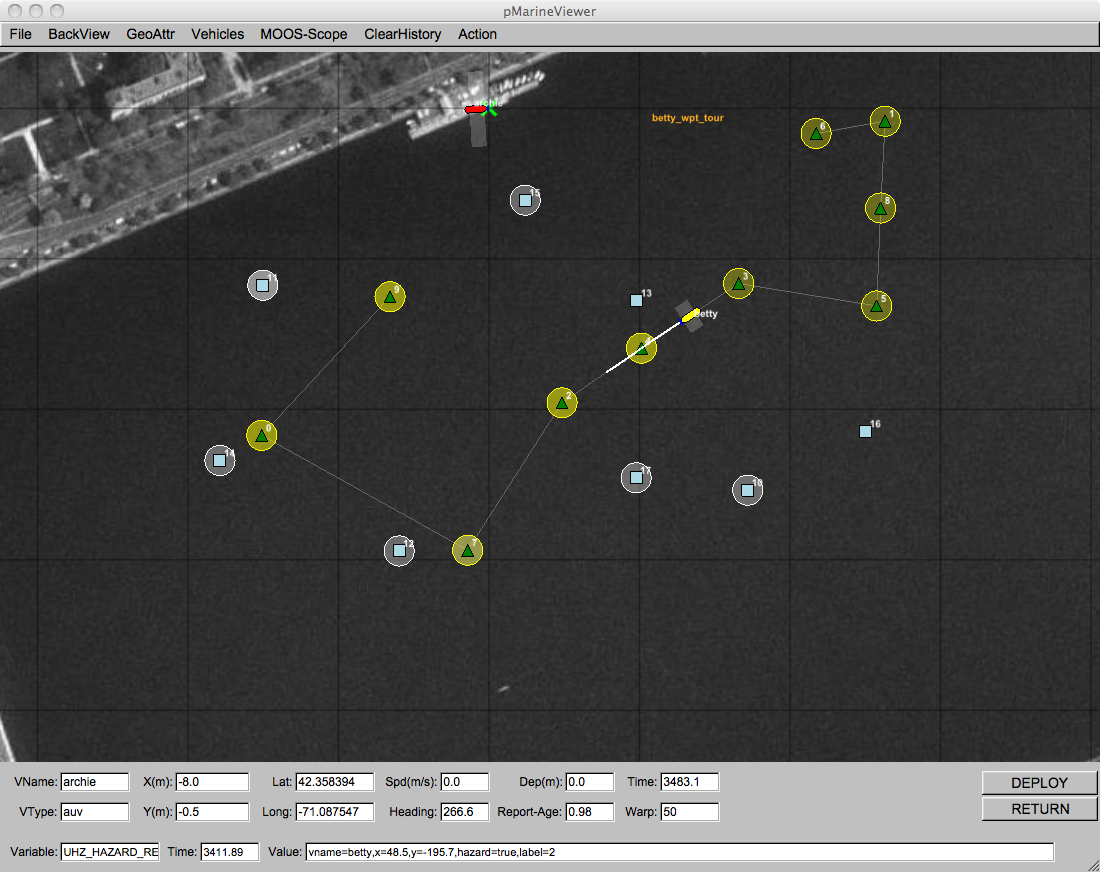
Figure 13.2: A Reacquire Mission: A second vehicle revisits a set of previously detected objects and seeks to reduce the uncertaintly associated with their initial classification made with a less reliable sensor.
In this mission, the vehicle's sensor is configured with a swath width of 10 meters (5 meters on either side), a probability of detection PD=0.9, probability of false alarm PFA=0.53, and probability of correct classification PC=0.93.
Document Maintained by: mikerb@mit.edu
Page built from LaTeX source using texwiki, developed at MIT. Errata to issues@moos-ivp.org. Get PDF