The alogview Tool for Analyzing Mission Log Files
Maintained by: mikerb@mit.edu  Get PDF
1 Overview
2 The Five Primary Viewing Windows
3 The NavPlot Window and Controlling Replay
3.1 Controlling the Current Time in Paused Mode
3.2 Controlling the Current Time in Streaming Mode
4 Background Region Images
4.1 Default Packaged Images
4.2 Image File Format and Meta Data (Info Files)
4.3 Obtaining Image Files
4.4 Loading Images at Run Time
4.5 Automatic alogview Detection of Background Image
4.6 Background Image Path
4.7 Troubleshooting
4.7.1 pMarineViewer fails to load the image (see only gray screen)
4.7.2 pMarineViewer or alogview image is fine but no vehicles
4.7.3 alogview fails to load the image (see only gray screen)
5 Video Capture
6 The LogPlot Window For Viewing Time-Series Data
6.1 Additional Buried but Useful Hot-Keys in the LogPlot Window
7 The IPFPlot Window For Viewing Helm Objective Functions
7.1 Launching an IPFPlot Window
7.2 Stepping Through Time and Replay Control in the IPFPlot Window
7.3 Selecting the IvP Function in the IPFPlot Window
7.4 Rendering the Collective IvP Function in the IPFPlot Window
7.5 Variable Scoping Within the IPFPlot Window
7.6 Additional Buried but Useful Hot-Keys in the IPFPlot Window
8 The HelmPlot Window For Viewing Helm State
8.1 Launching the HelmPlot Window
8.2 Stepping Through Time and Replay Control in the HelmPlot Window
8.3 Behavior States in the Helm Plot Window
8.4 Behavior Warnings, Errors, Mode History and Life Events
8.5 Additional Buried but Useful Hot-Keys in the HelmPlot Window
9 The VarPlot Window For Viewing Variable Histories
9.1 Launching the VarPlot Window
9.2 Viewing the Variable History in the VarPlot Window
9.3 Adding and Removing Variables from the History List
9.4 Additional Buried but Useful Hot-Keys in the VarPlot Window
10 Command Line Usage for the alogview Tool
1 Overview
The alogview application is a post-mission analysis utility loaded with one or more alog files, typically one per vehicle. It is more than a log file playback tool. A full state is maintained across all vehicles for both playing back sequentially and rewinding or jumping to any arbitrary point in time. The main window may look a bit like the run-time pMarineViewer window, but many of the GUI components in alogview are available solely for post-mission analysis. A snapshot of the tool, with no pop-up sub-windows open, is shown in Figure 1.1.

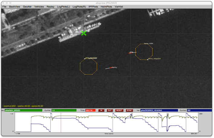
Figure 1.1: The alogview tool: used for post-mission rendering of alog files from one or more vehicles and stepping through time to analyze helm status, IvP objective functions, and other logged numerical data correlated to vehicle position in the op-area and time.
Quick Start: Launch alogview with one or more alog files on the command line, for example the two vehicle alog files from the m2_berta example mission:
$ alogview henry.alog gilda.alog
Upon launch, the viewer should look similar to Figure 1.1. Step forward or backward through time with the '[' or ']' keys, or click anywhere in the time-series in the bottom part of the screen. Replay can also be automated by accelerating or decelerating replay with the 'a or 'z' characters. Many other replay and visualization options are available via the pull-down menus and are introduced in later sections.
Recent History of Development with Releases
- Pre-2011: This tool existed as logview, was not documented and had limited support for rendering objective functions and helm information. Mostly used in-house by developers.
- 2011: Better support for IvP function rendering. Initial thin documentation. Support added for geometric log entries. Still very buggy but useful enough to share with other adventurous users. Biggest limitations: (a) initial full-alog load into memory too huge for anything but small missions. (b) no general scoping tool available for non-numerical data, (c) many little bugs or incomplete features.
- 2015: First real attempt to support users generally outside core developers. Better memory management for large and/or multi-vehicle missions. New scope for non-numerical data. Pop-up implementation of sub-windows. Unlimited sub-windows supported for multi-vehicle missions. Overall much less buggy and more feature-rich.
2 The Five Primary Viewing Windows
The alogview tool can be described by its five GUI components, listed below. The first two are always open upon startup, and the remaining three are upon user request via the pull-down menus:
- The NavPlot window: This is the main vehicle viewing area shown at the top in Figure 1.1. It primarily shows the current vehicle position(s) and perhaps recent trajectory and other geometric artifacts produced by the vehicle apps or behaviors, such as waypoints or sensor artifacts. More detail in Section 4.
- The LogPlot window: This is the time-series window shown at the bottom in Figure 1.1. The variable's rendered are selected by the user from the list any logged numerical data from any vehicle. More detail in Section 7.
- The IPFPlot window: (pronounced "i-p-f-plot") This is a pop-up window launched from the IPFPlots pull-down menu, for a chosen vehicle. It will render the prevailing IvP objective functions responsible for latest helm decision. More detail in Section 8.
- The HelmPlot window: This is a pop-up window launched from the HelmPlots pull-down menu, for a chosen vehicle. It shows the helm state in terms of active, running, idle behaviors, as well as behavior warnings, errors and life events. More detail in Section 9.
- The VarPlot window: This is a pop-up window launched from the VarPlots pull-down menu, for a chosen vehicle, and chosen logged MOOS variable (string or double). It shows an ordered list of recent and pending postings for the given variable. Additional variables can be added resulting in an interleaved sequence. More detail in Section 10.
In all windows, the current time can be altered with the same keyboard hot keys, found in the Replay pull-down menu and described in Section 4.
3 The NavPlot Window and Controlling Replay
The NavPlot window is the main viewing space, shown upon startup, with the current and recent vehicle positions rendered for each vehicle alog file. It is the top part shown in Figure 1.1.

3.1 Controlling the Current Time in Paused Mode [top]
By default alogview is paused upon startup. The options for stepping forward and backward through time may be seen from the Replay pull-down menu. There are three pairs of options:
- The '[' and ']' keys for stepping forward and backward by 1 second.
- The '{' and ''} keys for stepping forward and backward by 5 seconds.
- The 'ctrl-[' and 'ctrl-]' keys for stepping forward and backward by 0.1 seconds.
3.2 Controlling the Current Time in Streaming Mode [top]
Replay may also be put into a streaming mode at any time by accelerating or decelerating the streaming speed. Streaming is controlled by the following three keys:
- The 'a' key will accelerate the time warp, doubling the warp upon each successive hit, up to 64Hz.
- The 'z' key will decelerate the time warp, halving the warp upon each successive hit, down to 1/8Hz.
- The 'SPACEBAR' key will pause or unpause the streaming mode at any time.
The time warp is always shown in the very top of the alogview window. When streaming at say 16Hz, you should see (Time Warp = 16) in the window title bar. When not streaming, i.e., paused, this is indicated instead of the time warp, as in Figure 1.1.
Note that in streaming, between each update, there is work going on under the hood in addition to the rendering tasks. This includes the update of the current state of what is being rendered in the main and pop-up windows. Often it is not possible to refresh at the time warp requested. In this situation, alogview, and your machine, will do the best it can to keep up. Instead of seeing (Time Warp = 16) in the title bar, you may see something like (Time Warp = 16)(Actual:8.73). The latter number will vary, but represents the best warping rate possible given what is being updated between refreshes.
A faster observed time warp can be achieved by altering the streaming redraw interval. By default this interval is 0.5 seconds. So, for example, if the replay time warp is 4, then 8 re-draws will need to be handled per second. This may or may not be achievable. If the redraw interval is instead 1.0 seconds, then half as many re-draws are required for the same effective time warp. The drawback will be that the motion of the vehicle and objects will appear more "jumpy". The streaming redraw interval may be altered in the Replay pull-down menu.
4 Background Region Images
In both pMarineViewer and alogview, typical use involves a background region image upon which vehicles and other geometric objects are overlayed. Both utilies can be configured to use images of their own choosing. See examples in Figure 5.1. The user provides these images from whatever source they wish. Options for obtaining images and proper format are discussed below in the section Obtaining Image Files.
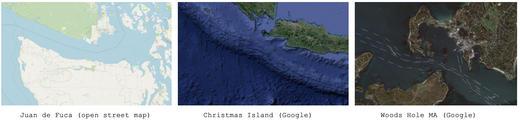
Figure 5.1: Example Background Region Images: The example images downloaded from freely available tile servers that may be utilized in either pMarineViewer or alogview.
4.1 Default Packaged Images [top]
Image files can be large, and of course there are endless possibilities depending on where you are operarating and which kind of background images you prefer. That being said, a couple images are distributed with MOOS-IvP. This allows example missions distributed with the MOOS-IvP code to having working images out-of-the-box without requiring the new user to fetch images. These two images are for (a) the MIT Sailing Pavilion, and (b) Forest Lake in Gray Maine, the site of some of the earliest in-water experiments circa 2004. This files are:
- MIT_SP.tif
- forrest19.tif
Both are distributed with MOOS-IvP and can be found in moos-ivp/ivp/data. When pMarineViewer or alogview is launched, this directory will be examined for the specified image file. Instructions for loading user-provided images is are given below in section Loading Images at Run Time.
4.2 Image File Format and Meta Data (Info Files) [top]
Images loaded into pMarineViewer and alogview are in the format of "Tiff" files. These files have the suffix ".tif". Tiff files have been around since the eighties, use lossless compression, are typically high quality, but are not as common as formats such as jpeg. There are many freely available tools for converting back and forth between tiff and jpeg and other formats. Tiff files are used in pMarineViewer and alogview primarily due to the availability of the libtiff library, readily available through package managers on both the MacOS and Linux platforms.
Each .tif file used in pMarineViewer and alogview has a corresponding .info file, containing (a) the latitude and longitude coordinates of the image edges, and (b) the datum, or (0,0) coordinate, on the image. For example, the MIT_SP.tif file has a corresonding MIT_SP.info file found in the same directory.
 lat_north = 42.360264
 lat_south = 42.35415
 lon_east  = -71.080058
 lon_west  = -71.094214
 datum_lat = 42.358436
 datum_lon = -71.087448
4.3 Obtaining Image Files [top]
Image files may be obtained and used in pMarineViewer and alogview from any source convenient to the user. This includes opening an image in say Google Maps on a web browser and performing a screen grab. The drawback of this method however is that it may be hard to precisely determine the lat/lon coordinates of the edges used in the corresponding .info file.
There are several open tile servers which allow a user to download an image tile, or set of tiles, provided with a range of lat/lon coordinates. These tiles can then be stitched together to make a single image. Although this sounds cumbersome, this process can be automated in a script. One such script is Anaxi Map, written by Conlan Cesar:
https://github.com/HeroCC/AnaxiMap
This utility is capable of using one of several tile servers with various background styles, such as Google Maps, maps with terrain or bathymetry information, or maps with street data. See Figure 5.1.
AnaxiMap, or similar utilities, may produce images in jpeg or png format. MacOS and Linux provide native utilities for converting the format, or "exporting" the file, to tiff format. On MacOS or Linux, if the free ImageMagick package is installed, you can use the "convert" utility:
$ convert region.jpg region.tif
4.4 Loading Images at Run Time [top]
Post Release 22.8, both pMarineViewer and alogview support operation with multiple background images. Toggling between images at run time is done by selecting the BackView pull-down menu and selcting tiff_type toggle, or by simply hitting the ` (back-tick) key.
In pMarineViewer, the multiple background images may be specified with multiple configuration lines, for example:
  tiff_file  = MIT_SP.tif
  tiff_file  = mit_sp_osm18.tif
In alogview, the multiple background images may be specified on the command line:
$ alogview --bg=MIT_SP.tif --bg=mit_sp_osm18.tif file.alog
4.5 Automatic alogview Detection of Background Image [top]
When launching alogview typically the user wants to use the same background region image used by pMarineViewer during the course of the mission that generated the alog file. In a new feature, post Release 22.8, alogview will automatically attempt to detect the image file used by pMarineViewer. The name name of region image is now published by pMarineViewer during the execution of the mission. This information is contained in the variable REGION_INFO. For example:
   REGION_INFO = lat_datum=42.358436, lon_datum=-71.087448, img_file=MIT_SP.tif,\
                 zoom=2.5, pan_x=129, pan_y=-364
The region info contains the name of the image (tiff) file used during the course of the mission, as well as the pan and zoom information as hints for alogview for use upon startup. The images found in REGION_INFO in the alog file will be loaded, as well as any images specified on the command line with the --bg options.
4.6 Background Image Path [top]
Support for the IVP_IMAGE_DIRS shell path is a new feature, post Release 22.8, relevant to both pMarineViewer and alogview. This is explained below.
Image files are named in either the pMarineViewer config block of the .moos mission file, or named on the command line when launching alogview, as specified in Section Loading Images at Run Time. For alogview, the file may also be named in the REGION_INFO logged variable as discussed above.
Both apps need to find the named .tif file. When found, it looks for the corresponding .info file in the same directory. There are four options for making this work:
- The image file is in the same directory as the mission file.
- The image file is in the special directory moos-ivp/ivp/data.
- The full or relative path name of the file is specified.
- The file exists in a directory on your IVP_IMAGE_DIRS path.
The first option has the drawback of duplicating the image file in potentially many places. The second option has the drawback that the directory moos-ivp/ivp/data is part of the MOOS-IvP code distribution which users otherwise consider to be read-only. A fresh check out of MOOS-IvP would reset this directory and users would need to take care to migrate files to a new checkout. The third option is that full or relative path name may not be the same between different users or machines. The fourth option is the newest option and arguably has the least downside.
The IVP_IMAGE_DIRS is shell (e.g., bash) environment variable. It contains a list of one or more directories on your local computer where pMarineViewer or alogview will look when attempting to load image files. Shell environment variables are already common settings that users will customize on their particular machine.
The recommended way for users to use a set of custom image files is to (a) organize them in one or more directories, preferably under version control, (b) install them at a convenient location on your local machine, (c) configure the IVP_IMAGE_DIRS shell variable to contain the one or more directories where your image files reside.
For example, if you have a folder of image files with the following structure:
   my_images/
      napa_bay/
         napa_bay_gmaps.tif
         napa_bay_gmaps.info
         napa_bay_osm.tif
         napa_bay_osm.info
      happy_harbor/
         happy_harbor_gmaps.tif
         happy_harbor_gmaps.info
         happy_harbor_osm.tif
         happy_harbor_osm.info
If this folder is installed on your machine in the home dirctory folder call "project", then you would set your IVP_IMAGE_DIRS path in your shell configuration file, e.g., .bashrc, as follows:
   IVP_IMAGE_DIRS=~/project/napa_bay
   IVP_IMAGE_DIRS+=:~/project/happy_harbor
To verify which file has been loaded, the appcasing output of pMarineViewer shows the full path name of the loaded file(s). And when alogview is launched, the terminal output indicates which directories are being searched, in order, for the image files. This information may be obscured however when the alogview window pops up, but you can find it if you go back to it and perhaps scroll up. Note: It is not sufficient, in the example above, to simply set IVP_IMG_DIR=~/project, the parent directory of all image folders. Each image folder must be named.
4.7 Troubleshooting [top]
4.7.1 pMarineViewer fails to load the image (see only gray screen) [top]
- Check the appcasting output of pMarineViewer. The top few lines should show which image file is loaded. Is this a file you recognize?
- Does this file exist on your computer? Verify it is where you think it is.
- How are you specifying this file in your pMarineViewer config block? If it is specified as a relative path, e.g., ../my_images/napa_bay.tif, make sure that relative path location is correct.
- If you are specifying the image file with just the file name (no path information), then check you have your IVP_IMAGE_DIRS variable set properly. Run echo $IVP_IMAGE_DIRS on the command line.
- Simplest but most common: Make sure your image file name (configuration and actual name) end in the suffix .tif and not .tiff.
4.7.2 pMarineViewer or alogview image is fine but no vehicles [top]
- Check the .info file. Make sure the lat/lon values sanity check, e.g., rough magnitude, relative values.
- Make sure the datum_lat and datum_lon values are in the range of the image.
- Make sure the datum_lat and datum_lon values match the datum set at the top of the vehicle and shoreside mission files.
4.7.3 alogview fails to load the image (see only gray screen) [top]
In the newer version of alogview, when launching it will attempt to read the name of the image file used by pMarineViewer. So if pMarineViewer launched ok, chanches are good alogview will also launch with the same image. However, it could be the case that (a) the mission was run on some other computer that contained the image file and your current computer does not. The image file is not logged. (b) the mission was named
- Does this file exist on your computer? Verify it is where you think it is. It is possible that you are trying to run alogview on your computer with alog files generated on someone else's computer. Make sure you have the image file.
- Check the terminal output of alogview as it is loading. To demonstrate the below output from an alogview launch purposely use the the file dforrest19.tif instead of forrest19.tif. Note the sequences of folders searched in the attempt to find the image file. The first attempt is the in the moos-ivp/ivp/data directory. The next attempts are based on the value of IVP_IMAGE_DIRS. The final attempt is in the current working directory where alogview was launched. Does this match up with your expectations?
 TIFF FILES COUNT:1
 [1] Looking for dforrest19.tif and dforrest19.info in:
 Dir: [/Users/james/moos-ivp/ivp/data]
 Not found.
 [2] Looking for dforrest19.tif and dforrest19.info in:
 Dir: [/Users/james/pavlab_map_images/popolopen]
 [3] Looking for dforrest19.tif and dforrest19.info in:
 Dir: [/Users/james/pavlab_map_images/mit]
 [4] Looking for dforrest19.tif and dforrest19.info in:
 Dir: [/Users/james/moos-ivp/ivp/datax]
 [5] Looking for dforrest19.tif and dforrest19.info in:
 Dir: [/Users/james/moos-ivp/ivp/data-local]
 [6] Looking for dforrest19.tif and dforrest19.info in:
 Dir: [/Users/james/moos-ivp/ivp/data]
 [*] Looking for dforrest19.tif and dforrest19.info in:
 Dir: [./]
 Not found.
 Could not find the pair of files:
 dforrest19.tif and dforrest19.info
 Opening Tiff:
 TIFFOpen: : No such file or directory.
 Failed!!!!!!!!!
- Simplest but most common: Make sure your image file name (configuration and actual name) end in the suffix .tif and not .tiff.
5 Video Capture
Video capture is no longer natively supported in alogview due to the common availability of third party video capturing software. Just launch alogview, put it into streaming mode (Section 4.2) at the desired rate, and launch your favorite video capture program.
6 The LogPlot Window For Viewing Time-Series Data
The LogPlot window allows the rendering of any numerical data from any loaded alog file to be plotted against time, as shown in Figure 1.1 and up close in Figure 7.1 below. The user may zoom in to see finer resolution in the postings, by clicking either the IN or OUT buttons, or by the 'i' or 'o' keys while the mouse is in the LogPlot window. To return to the original full apperature zoom, hit the RESET button. The user may left-click at any point in the time series to adjust the current time (shown by the red bar in the viewer). This time adjustment is propagated not only to the NavPlot viewer but to all open pop-up windows.
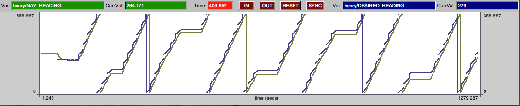
Figure 7.1: The logplot window: is used for viewing any numerical data found in any of the alog files loaded into alogview. Here the desired and actual vehicle headings are logged side-by-side.
Two variables, and two y-axes are available for selection. By default they are drawn on independent scales to allow variables with starkly different ranges, such as speed and heading, to be meaningfully rendered. The user may choose to synchronize the two variable ranges rendered to allow for more meaningful comparisons when the two variables have the same range, such as desired and observed speed. The synchronization is done by hitting the SYNC button at the top of the logplot window. The user chooses which two variables are rendered from the pull-down menu as shown in Figure 7.2.
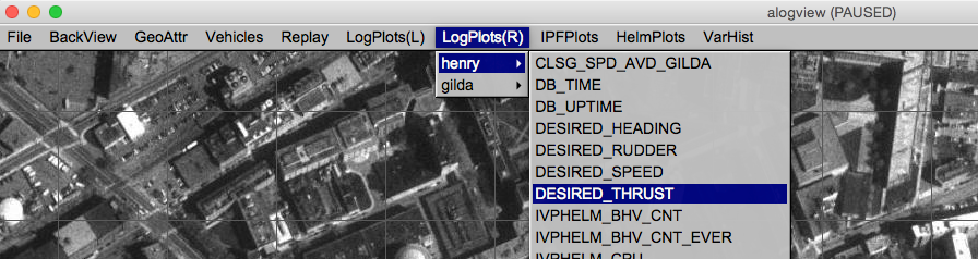
Figure 7.2: The logplot pull-down menu: is used for first selecting the vehicle and then the variable to be plotted.
If you find yourself wanting to repeatedly open an alog file with same one or two variables chosen for the LogPlot window, these variables can be chosen and at launch time passed as command line arguments:
$ alogview --lp=henry:NAV_SPEED --rp=gilda:NAV_SPEED
6.1 Additional Buried but Useful Hot-Keys in the LogPlot Window [top]
There are a few hot-key functions available (only when the main window is active and the mouse is over the LogPlot window, that may not be apparent from simply interacting with the window:
- The 'i' key: will zoom in the resolution on the plot. This can also be done by hitting the IN button.
- The 'o' key: will zoom out the resolution on the plot. This can also be done by hitting the OUT button.
- The 'LEFT' and 'RIGHT' keys: will step forward and backward through time by 1 second.
- The 'UP' and 'DOWN' keys: will zoom in and out on the plot, essentially the same as the 'i' and 'o' keys.
The above hot-keys are in addition to the time control hot-keys listed in Section sec_alv_time_replay and Section 4.1.
7 The IPFPlot Window For Viewing Helm Objective Functions
The IPFPlot window allows the rendering of an IvP function (IPF) from any vehicle and any behavior found in any of the alog files loaded into alogview.
7.1 Launching an IPFPlot Window [top]
An IPFPlot pop-up window is launched from the alogview main pull-down window as shown in Figure 8.1, by choosing a vehicle name. Separate windows can be opened for different vehicles, or even for the same vehicle.
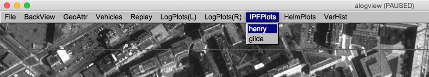
Figure 8.1: The ipfplot pull-down menu: is used for first selecting the vehicle and then the variable to be plotted.
A newly launched pop-up window loads the relevant information from disk into the alogview memory space. This includes all IvP functions for all behaviors at all times, for the given vehicle. This can be large. For some (larger) missions and some computer configurations, the larger memory footprint will begin to be noticed in terms of application responsiveness. Likewise, the internal data structure updates, each time the current time is changed, increases for each pop-up window. This may result in a slower streaming rate when in replay. Closing the pop-up window releases the memory and should immediately boost responsiveness and playback rate.
7.2 Stepping Through Time and Replay Control in the IPFPlot Window [top]
The current time is shown in the upper left corner and is synchronized with the main viewing window and any other pop-up windows that may be open. The same time keys are functional when this window is active, e.g., '[', ']', '{', ''}, for stepping forward and backward in time. The replay control keys, e.g., 'a', 'z', are also functional, and the replay state and rate is also shown in the title bar of this window.
7.3 Selecting the IvP Function in the IPFPlot Window [top]
The user may choose any single objective function at a time from the menu on the left side of the window shown in Figure 8.2. The current behavior weight is shown alongside the behavior name in the menu. If a behavior presently has a weight of zero, no function will be rendered when that behavior is selected. Multiple objective functions may be viewed simultaneously by launching more pop-up windows.
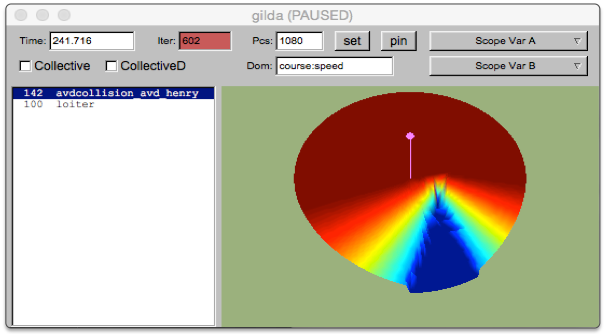
Figure 8.2: The ipfplot window: used for examining IvP functions for the chosen vehicle at the current time.
Since each window is associated with a particular vehicle, the helm iteration may be shown unambiguously in the redish window in the upper left. The rendering of the IvP function may be rotated or tilted for different perspectives by using the arrow keys. The perspective may be returned to the bird's eye view by hitting the SET button.
7.4 Rendering the Collective IvP Function in the IPFPlot Window [top]
IvP functions of two forms are renderable - those defined over course and speed, and those defined over depth. In both cases, a rendering of the collective function is possible by clicking on the Collective or CollectiveD check-boxes on the left. In Figure 8.3 below, the collective objective function is shown, showing the weighted sum of the two behaviors The purplish pin rendered in Figures 8.2 and 8.3 shows the actual chosen decision for the present helm iteration. When rendering the collective function as in Figure 8.3 the pin should be visually consistent with the peak of the function. When rendering a single objective function, as in Figure 8.2, the pin may not visually correlate to the peak of the function since other functions may be in play. For example in Figure 8.2 the pin identifies one of many points on the red plateau. The pin can be toggled on and off by hitting the PIN button.
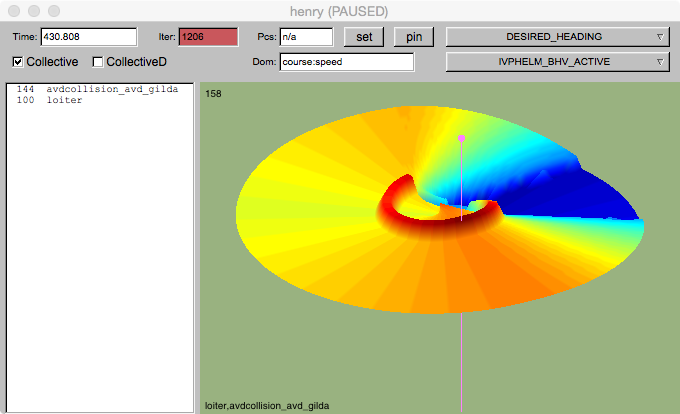
Figure 8.3: The ipfplot window: showing here the collective objective function representing the weighted sum of the two active behaviors.
7.5 Variable Scoping Within the IPFPlot Window [top]
Often it is useful to scope on a couple key variables related to the rendered objective function, to observe how they change and perhaps influence the function as time evolves. Although a general scoping ability exists via the VarPlot window described below in Section 10, it can be handy to see the variable value(s) right in the IPFPlot window. The two pull-down menu buttons in the upper right in Figure 8.3 allow the selection of two variables whose values are output in the upper and lower left hand corners of the window as shown. The choice of these two variables is specific to the chosen behavior, or collective function. A different set of variables my be associated with each behavior, and they will be refreshed accordingly as the user switches between behaviors.
7.6 Additional Buried but Useful Hot-Keys in the IPFPlot Window [top]
There are a few hot-key functions available that may not be apparent from simply interacting with the window:
- The '+' key: will increase the font size in the browser pane, and the font size of any scoped variable.
- The '-' key: will decrease the font size in the browser panes, and the font size of any scoped variable.
- The 'c' key: will toggle the IvP function rendering from an individual selected function to the collective objective function.
- The 'f' key: will put the window in a "full-window" mode showing only the rendered objective function, without the browser pane.
- The 'UP' and 'DOWN' keys: will tilt the rendered objective functions.
- The 'LEFT' and 'RIGHT' keys: will rotate the rendered objective functions.
The above hot-keys are in addition to the time control hot-keys listed in Section sec_alv_time_replay and Section 4.1.
8 The HelmPlot Window For Viewing Helm State
The HelmPlot window renders information regarding the present helm state, including which behaviors are in which state and for how long, summary of update attempts for each behavior, behavior warnings, behavior errors, a history of helm mode changes, and a history of helm life events.
8.1 Launching the HelmPlot Window [top]
The HelmPlot pop-up window is launched from the alogview main pull-down window as shown in Figure 9.1, by choosing a vehicle name. Separate windows can be opened for different vehicles, or even for the same vehicle.
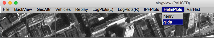
Figure 9.1: The helmplot pull-down menu: is used for first selecting the vehicle and launching the HelmPlot window.
A newly launched pop-up window loads the relevant information from disk into the alogview memory space. For some (larger) missions and some computer configurations, the larger memory footprint will begin to be noticed in terms of application responsiveness. Likewise, the internal data structure updates, each time the current time is changed, increases for each pop-up window. This may result in a slower streaming rate when in replay.
8.2 Stepping Through Time and Replay Control in the HelmPlot Window [top]
The current time is shown in the upper left corner and is synchronized with the main viewing window and any other pop-up windows that may be open. The same time keys are functional when this window is active, e.g., '[', ']', '{', ''}, for stepping forward and backward in time. The replay control keys, e.g., 'a', 'z', are also functional, and the replay state and rate is also shown in the title bar of this window.
8.3 Behavior States in the Helm Plot Window [top]
Each behavior known to the helm up to the present time is grouped into a list of either active, running, idle or completed modes as shown in Figure 9.2.
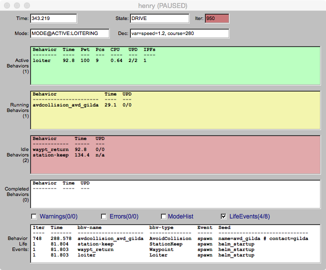
Figure 9.2: The helmplot window: used for analyzing the helm state and behavior modes.
For each behavior, the behavior name is listed, along with the elapsed time since the behavior has been in that mode. If the behavior is configured with the updates parameter, then the number of successful vs attempted updates are also listed. If the behavior does not have the updates parameter set, then n/a will instead be listed in that column as with the station-keep behavior in the figure below. For active, behaviors, the present priority weight and number of pieces is also shown.
8.4 Behavior Warnings, Errors, Mode History and Life Events [top]
The bottom pane of the HelmPlot window may have one of four content modes, selectable with the check-box shown.
- Behavior Warnings: In this mode, all behavior warnings, in the form of messages written to BHV_WARNING, will be listed in chronological order with the most recent at the top. One handy feature is that the existence of possible future warnings can be see in the check-box label. In parentheses, (a/b) indicates that a warnings are shown in the list out of b warnings total for the mission.
- Behavior Errors: In this mode, all behavior errors, in the form of messages written to BHV_ERROR, will be listed in chronological order with the most recent at the top. In the check-box label, in parentheses, (a/b) indicates that a errors are shown in the list out of b errors total for the mission.
- Mode History: In this viewing mode, all helm mode changes will be listed in chronological order with the most recent at the top.
- Life Events: In this viewing mode, all helm life events (behavior spawning and deaths) will be listed in chronological order with the most recent at the top.
8.5 Additional Buried but Useful Hot-Keys in the HelmPlot Window [top]
There are a few hot-key functions available that may not be apparent from simply interacting with the window:
- The '+' key: will increase the font size in the browser pane, and the font size of any scoped variable.
- The '-' key: will decrease the font size in the browser panes, and the font size of any scoped variable.
- The 'UP' and 'DOWN' keys: will tilt the rendered objective functions.
- The 'LEFT' and 'RIGHT' keys: will rotate the rendered objective functions.
The above hot-keys are in addition to the time control hot-keys listed in Section sec_alv_time_replay and Section 4.1.
9 The VarPlot Window For Viewing Variable Histories
The VarPlot window renders the full history of one or more chosen MOOS variables, allowing the user to see the present value, recent postings, and upcoming pending postings. This holds for both numerical and string variables.
9.1 Launching the VarPlot Window [top]
The VarPlot pop-up window is launched from the alogview main pull-down window as shown in Figure 10.1, by choosing a vehicle name, and MOOS variable name. Separate windows can be opened for different vehicles, variables, or even for the same vehicle and variable. Although one variable is chosen upon launch, any number of variables can be inserted later from the VarPlot pull-down buttons
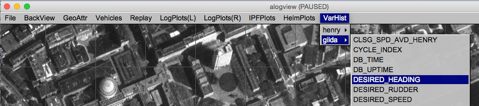
Figure 10.1: The VarPlot pull-down menu: is used for first selecting a vehicle and variable name, and launching the VarPlot window.
A newly launched pop-up window loads the variable history information from disk into the alogview memory space. For some (larger) missions and some computer configurations, the larger memory footprint will begin to be noticed in terms of application responsiveness. Likewise, the internal data structure updates, conducted each time the current time is changed, increases for each pop-up window. This may result in a slower streaming rate when in replay. Closing the pop-up window releases the memory and should immediately boost responsiveness and playback rate.
9.2 Viewing the Variable History in the VarPlot Window [top]
The VarPlot window contains two primary panes. The top pane shows everything in the past, up to the most recent post. The bottom pane shows everything in the future, starting with the next pending post. The "current time" can be regarded as being in between the two panes.
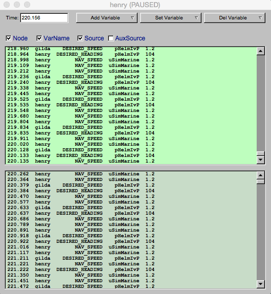
Figure 10.2: The VarPlot window: used for scoping on a set of MOOS variables into the past and upcoming in the future.
Each variable posting has six components, separated into six columns in both panes:
- Time: The timestamp of the posting. This is always shown in the first column.
- Node: The node, i.e., vehicle name is shown in the second column. Since the scope may contain values across nodes, this can be useful to see. If only scoping on one variable, or if all variables are from the same node, then this column can be hidden by toggling the Node check-box.
- Variable Name: If scoping on only one variable, this third column may be hidden to provide more visibility to the other columns.
- Source: The source, i.e., MOOS App that generated the posting, is shown in the fourth column. This may be toggled on or off.
- Auxiliary Source: The auxiliary source is shown in the fifth column. Most MOOS apps do not make postings with an auxiliary source. The helm does however, and this typically indicates the particular behavior that produced the posting.
- Variable Value: The last column is just the value of the posting. This column cannot be hidden.
9.3 Adding and Removing Variables from the History List [top]
Upon launching the VarPlot window, a single variable is chosen. After launching, additional variables may be added (from any vehicle) from the Add Variable pull-down menu button as shown in Figure 10.3. The Set Variable button presents the same set of choices, but will essentially remove all previously selected variables and replace it with the chosen one. The Del Variable button will remove the selected variable from the current set of variables.
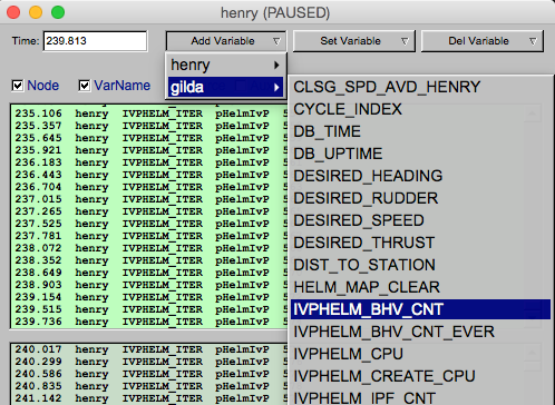
Figure 10.3: The VarPlot window: Any variable from any vehicle may be added any time after the window is opened.
9.4 Additional Buried but Useful Hot-Keys in the VarPlot Window [top]
There are a few hot-key functions available that may not be apparent from simply interacting with the window:
- The '+' key: will increase the font size in the browser panes.
- The '-' key: will decrease the font size in the browser panes.
The above hot-keys are in addition to the time control hot-keys listed in Section sec_alv_time_replay and Section 4.1.
10 Command Line Usage for the alogview Tool
The alogview tool is run from the command line with one or more given .alog files and a number of options. The usage options are listed when the tool is launched with the -h switch:
$ alogview --help or -h
Listing 11.1 - Command line usage for the alogview tool.
    1  Usage:
    2    alogview file.alog [another_file.alog] [OPTIONS]
    3
    4  Synopsis:
    5    Renders vehicle paths from multiple MOOS .alog files. Replay
    6    logged data or step through manually. Supports several
    7    specialized pop-up windows for viewing helm state, objective
    8    functions, any logged variable across vehicles. If multiple
    9    alog files are given, they will synchronized. Upon launch,
   10    the original alog files are split into dedicated directories
   11    to cache data base on the MOOS variable name.
   12
   13  Standard Arguments:
   14    file.alog - The input logfile.
   15
   16  Options:
   17    -h,--help       Displays this help message
   18    -v,--version    Displays the current release version
   19
   20    --bg=file.tiff  Specify an alternate background image.
   21
   22    --lp=VEH:VAR    Specify starting left log plot.
   23    --rp=VEH:VAR    Specify starting right log plot.
   24                    Example: --lp=henry:NAV_X
   25                    Example: --rp=NAV_SPEED
   26
   27    --nowtime=val   Set the initial startup time
   28    --mintime=val   Clip all times/vals below this time
   29    --maxtime=val   Clip all times/vals above this time
   30
   31    --quick,-q      Quick start (no geo shapes, logplots)
   32    --altnav=PREF   Alt nav solution prefix, e.g., NAV_GT_
   33
   34    --zoom=val      Set initial zoom value (default: 1)
   35    --panx=val      Set initial panx value (default: 0)
   36    --pany=val      Set initial pany value (default: 0)
   37
   38    --geometry=xsmall  Open GUI with dimensions 770x605
   39    --geometry=small   Open GUI with dimensions 980x770
   40    --geometry=medium  Open GUI with dimensions 1190x935
   41    --geometry=large   Open GUI with dimensions 1400x1100
   42    --geometry=WxH     Open GUI with dimensions WxH
   43
   44  Further Notes:
   45    (1) Multiple .alog files ok - typically one per vehicle
   46    (2) See also: alogscan, alogrm, alogclip, aloggrep
   47        alogsort, alogiter, aloghelm
The order of the arguments passed to alogview do not matter. The --mintime and --maxtime arguments allow the user to effectively clip the alog files to reduce the amount of data loaded into RAM by alogview during a session. The --geometry argument allows the user to custom set the size of the display window. A few shortcuts, "large", "medium", "small", and "xsmall" are allowed.
Page built from LaTeX source using texwiki, developed at MIT. Errata to issues@moos-ivp.org. Get PDF