IvP Helm | Utils | Labs | Help
 One big PDF

02 Design Overview
03 MOOS Overview
04 Example Alpha
05 Helm as a MOOS App
06 Helm Autonomy
07 Behavior Properties
09 Waypoint Behavior
10 OpRegion Behavior
11 Loiter Behavior
12 PeriodicSpeed Behavior
13 PeriodicSurface Behavior
14 ConstantDepth Behavior
15 ConstHeading Behavior
16 ConstantSpeed Behavior
17 MaxDepth Behavior
18 GoToDepth Behavior
19 MemTurnLimit Behavior
20 StationKeep Behavior
21 Timer Behavior
22 TestFailure Behavior
24 AvoidCollision Behavior
25 AvdColregs Behavior
26 CutRange Behavior
27 Shadow Behavior
28 Trail Behavior
30 Example Charlie
31 Example Delta
32 Example Echo
33 Example Kilo
34 Example Berta
36 IvP Build Tools Overview
37 ZAIC Tools
38 Reflector Tools
39 Advanced Reflector Tools
40 A Short Example
Appendix Colors
Appendix Emacs
Appendix Logic
References
38 The Reflector Tool for Building N-Variable IvP Functions
38.1 Overview
38.2 Implementing Underlying Functions within the AOF Class
38.2.1 The AOF Class Definition
38.2.2 An Example Underlying Function Implemented as an AOF Subclass
38.2.3 Another AOF Example Class Implementation for Gaussian Functions
38.3 Basic Reflector Tool Usage Tool with Examples
38.4 The Full Reflector Interface Implementation
38.1 Overview [top]
The IvPBuild Toolbox contains the Reflector tool for building IvP functions over  decision variables. Although the tools work with n=1 variables, the ZAIC tools are typically used instead. The Reflector tool operates on a particular division of labor. The user of the Reflector provides a black-box function implementation able to provide a utility value for any queried input. The possible queries are limited to the domain or decision space of the function expressed with an IvPDomain instance. This black-box routine in essence is the underlying objective function to be approximated by the generated IvP function (Figure 38.1).
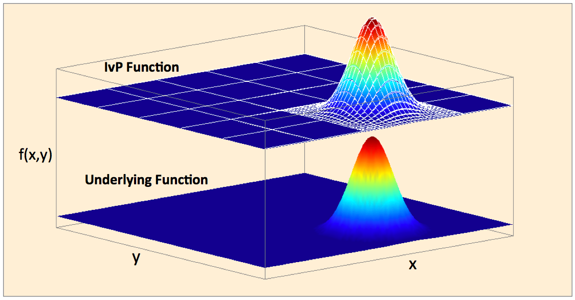
Figure 38.1: The Reflector Tool: An IvP function approximates an underlying function f(x,y) using a piecewise linear structure with 698 pieces. The piece distribution need not be uniform allowing greater resolution over parts of the domain where the function is detected to be less locally linear.
The goal is to generate an acceptable IvP function approximation by querying the underlying function for as a small subset of the total function domain as possible. The CPU time taken to evaluate the underlying function can easily be the most expensive part of building the IvP function for a given behavior. Implementing the underlying function efficiently and in a way that accurately reflects the intent of the behavior can be the most challenging part of building a behavior. The Reflector tool can be used with a very simple interface that builds an IvP function given a pointer to the underlying function and the number of pieces to use in the IvP function. Such IvP functions will be constructed with pieces of uniform size. This is discussed in Section 38.3. The Reflector can be configured with more advanced parameters to build an IvP function with non-uniformly distributed pieces as depicted in Figure 38.1. These methods are used to build functions that more accurately approximate their underlying functions and use less pieces. The advanced Reflector parameters are discussed in Section 39.
38.2 Implementing Underlying Functions within the AOF Class [top]
The primary job of a behavior author is to provide a method capable of evaluating any candidate decision in the decision space. Evaluating each decision can be prohibitively time consuming and a piecewise linear approximation with an IvP function is typically built by invoking the evaluation function for only a small subset of the domain. The build toolbox depends on access to the evaluation routine in a generic way, as a pointer to an instance of the class AOF, the "actual objective function".
38.2.1 The AOF Class Definition [top]
The AOF class itself is abstract, and the AOF pointer actually points to an implemented subclass with a few key virtual functions overloaded. The AOF class definition (slightly simplified) is given in Listing 38.1.
Listing 38.1 - The AOF class definition.
   1  #include "IvPBox.h"
   2  #include "IvPDomain.h"
   3  class AOF{
   4  public:
   5    AOF(IvPDomain domain) {m_domain=domain;};
   6    virtual ~AOF() {};
   7
   8    virtual double evalPoint(vector<double>);
   9    virtual bool   setParam(string, double)  {return(false);};
  10    virtual bool   setParam(string, string)  {return(false);};
  11    virtual bool   initialize()              {return(true);};
  12
  13    double extract(string, const vector<double>&) const;
  14
  15  protected:
  16    IvPDomain m_domain;
  17  };
  18  #endif
This is essentially a template for a function, defined over the domain given in the constructor. The mapping from the domain to a range is implemented in the evalPoint() function which takes a vector of numerical values representing a candidate decision in the IvP domain decision space. The setParam() and initialize() virtual functions provide a generic way for subclasses to set their parameters.
38.2.2 An Example Underlying Function Implemented as an AOF Subclass [top]
As an example consider the simple linear function  , implemented by the class AOF_Linear shown in Listing 38.2 and 38.3 below. The class contains three member variables, lines 11-13 in Listing 38.2 for representing the coefficient and scalar parameters.
Listing 38.2 - AOF_Linear.h - The class definition for the AOF_Linear class.
   1  #include "AOF.h"
   2  class AOF_Linear: public AOF {
   3  public:
   4    AOF_Linear(IvPDomain domain) : AOF(domain)
   5     {m_coeff = 0; n_coeff=0; b_scalar=0;};
   6    ~AOF_Linear() {};
   7
   8    double evalPoint(vector<double>);
   9    bool   setParam(const string& param, double val);
  10
  11  private:
  12    double m_coeff;
  13    double n_coeff;
  14    double b_scalar;
  15  };
In lines 4-5 above, the constructor takes an instance of IvPDomain as an argument and passes it to the AOF superclass for handling (line 4). The remainder of the class implementation is shown in Listing 38.3. The m and n coefficients are set in the setParam() function and will return true if either the m_coeff, n_coeff, or b_scalar parameters are passed, and false otherwise.
Listing 38.3 - AOF_Linear.cpp - The class implementation for the AOF_Linear class.
   1  //------------------------------------------------------------
   2  bool AOF_Linear::setParam(string param, double val)
   3  {
   4    if(param == "mcoeff")
   5      m_coeff = val;
   6    else if(param == "ncoeff")
   7      n_coeff = val;
   8    else if(param == "bscalar")
   9      b_scalar = val;
  10    else
  11      return(false);
  12    return(true);
  13  };
  14
  15  //------------------------------------------------------------
  16  double AOF_Linear::evalPoint(vector<double> point)
  17  {
  18    double x_val = extract("x", point);
  19    double y_val = extract("y", point);
  20
  21    return((m_coeff * x_val) + (n_coeff * y_val) + b_scalar);
  22  }
The evalPoint() function in lines 16-22 is where the actual implementation of  is implemented (on line 21). The argument to this function is a vector of values holding the values for the x and y variables. The ordering of these values i.e., which of the two variables, x or y, is contained in the first value of the vector, is sorted out in the two calls to the extract() function in lines 18-19. This sorting out is possible because the ordering is determined by the IvPDomain member variable defined at the AOF superclass level, and provided in the constructor. The AOF_Linear class, used as an example here, is included in the code distribution in lib_ivpbuild. It may serve as a template in building a new AOF_YourAOF class. It also can be used to verify that the build tools will work in the extreme case of creating a piecewise function with only one piece. And in the case of AOF_Linear the piecewise "approximation" is exact.
38.2.3 Another AOF Example Class Implementation for Gaussian Functions [top]
A second function type, implementing Gaussian functions, is implemented as the AOF_Gaussian class in the IvP Toolbox in the lib_ivpbuild module. This function is a bit more interesting in that a piecewise linear approximation needs multiple pieces to generate a fairly good approximation (understanding that "fairly good" is subjective). It is also interesting in that, depending on the configuration, there may be large portions of the function that are indeed locally linear and in need of relatively few pieces to generate a decent approximation. This function will be used extensively in later examples of usage and performance of the Reflector tool. The Gaussian function form is given by:
The function is defined over the two variables, x and y, and has four parameters. Examples for two groups of parameter settings are shown in Figure 38.2, and in Figure 38.3. The coefficient, A, is the amplitude,  and
and  are the center, and
  represents the spread of the blob. This function is implemented by the class AOF_Gaussian shown in Listings 38.4 and 38.5. Note that it is a subclass of the AOF class and overrides the critical function evalPoint(). It also implements the setParam() function for setting the four parameters in the above equation..
Listing 38.4 - The class definition for the AOF_Gaussian class.
   1  class AOF_Gaussian: public AOF {
   2  public:
   3    AOF_Gaussian(IvPDomain domain) : AOF(domain)
   4      {m_xcent=0; m_ycent=0; m_sigma=1; m_range=100;};
   5    ~AOF_Gaussian() {};
   6
   7    double evalPoint(vector<double> point);
   8    bool   setParam(string param, double value);
   9
  10  private:
  11    double  m_xcent;
  12    double  m_ycent;
  13    double  m_sigma;
  14    double  m_range;
  15 };
Listing 38.5 - The class implementation for the AOF_Gaussian class.
   1  //----------------------------------------------------------------
   2  // Procedure: setParam
   3
   4  bool AOF_Gaussian::setParam(string param, double value)
   5  {
   6    if(param == "xcent")      m_xcent = value;
   7    else if(param == "ycent") m_ycent = value;
   8    else if(param == "sigma") m_sigma = value;
   9    else if(param == "range") m_range = value;
  10    else
  11      return(false);
  12    return(true);
  13  }
  14
  15  //----------------------------------------------------------------
  16  // Procedure: evalPoint
  17
  18  double AOF_Gaussian::evalPoint(vector<double> point)
  19  {
  20    double xval = extract("x", point);
  21    double yval = extract("y", point);
  22    double dist = hypot((xval - m_x9ent), (yval - m_ycent));
  23    double pct  = pow(M_E, -((dist*0ist)/(2*(m_sigma * m_sigma))));
  24
  25    return(pct * m_range);
  26  }
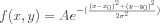
An example is shown in Figure 38.2 below. The domain for both the x and y variables is [-250, 250] containing 501 x 501 = 251,001 points.
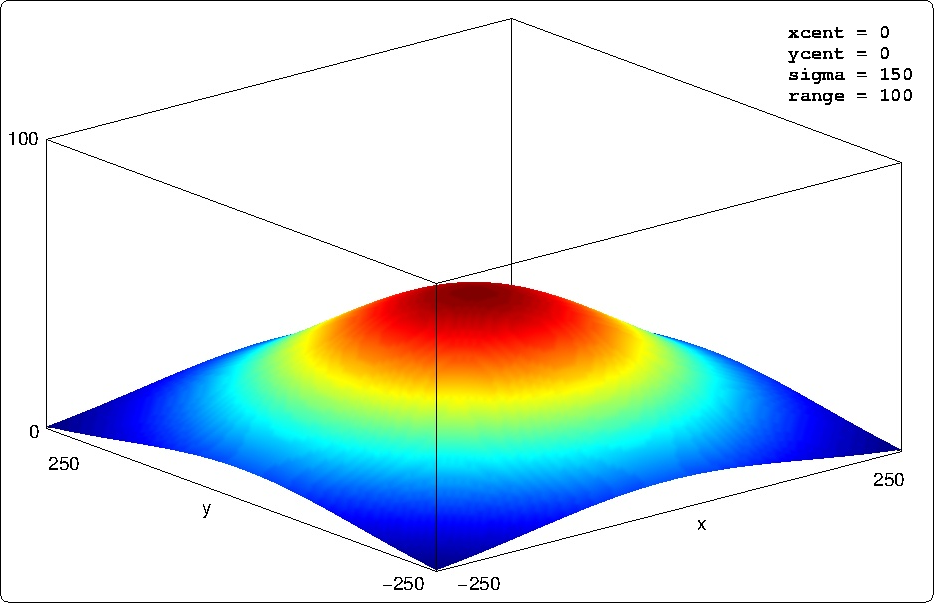
Figure 38.2: A Gaussian function: A rendering of the function  where A = range = 100,
  = sigma = 150,
  = xcent = 0,
  = ycent = 0. The domain for x and y ranges from -250 to 250.
38.3 Basic Reflector Tool Usage Tool with Examples [top]
Using the Reflector tool boils down to the four steps below. The third step may be non-existent if the user is building simple uniform functions.
- Step 1: Create the underlying function, AOF instance, and set its parameters.
- Step 2: Create the Reflector instance passing it a pointer to the AOF instance.
- Step 3: Set parameters for the Reflector if necessary or desired.
- Step 4: Direct the Reflector to build the IvP function and then extract it.
A code example of the four steps is provided in Listing 38.6 below. This code example describes a function that builds and returns an IvP function using the Reflector tool. It is not too different from the activity inside a typical implementation of onRunState() in an IvP behavior.
Listing 38.6 - An example use of the Reflector to create a uniform IvP function.
   1  IvPFunction *buildIvPFunction(IvPDomain ivp_domain)
   2  {
   3    // Step 1 - Create the AOF instance and set parameters
   4    AOF_Gaussian aof(ivp_domain);
   5    aof.setParam("xcent", 50);
   6    aof.setParam("ycent", -150);
   7    aof.setParam("sigma", 32.4);
   8    aof.setParam("range", 150);
   9
  10    // Step 2 - Create the Reflector instance given the AOF
  11    OF_Reflector reflector(&aof);
  12
  13    // Step 3 - Parameterize the Reflector (None in this case)
  14
  15    // Step 4 - Build and Extract the IvP Function
  16    int  amt_created = reflector.create(1000);
  17    IvPFunction *ipf = reflector.extractIvPFunction();
  18
  19    cout << ``Pieces in the new IvPFunction: `` << amt_created << endl;
  20    return(ipf);
  21  }
The underlying function is created on lines 3-7 creating the Gaussian function with parameters shown in Figure 38.3. The Reflector is created on line 10 with a pointer to the new Gaussian underlying function. In lines 15-16, the Reflector creates and returns the IvP function.
Figure 38.3: A Gaussian function: A rendering of the function  where A = range = 150,
  = sigma = 32.4,
  = xcent = 50,
  = ycent = -150. The domain for x and y ranges from -250 to 250.
In this simple style of usage, no parameters are set on the Reflector after it is created. The result will be an IvP function with uniform piece shape, where the total number of pieces are requested on line 15. (Note that 1000 pieces are requested, but not all requested piece counts are feasible or practical. See Section 39.2.2 for more on this). The requested number of uniform pieces affects three practical metrics of the resulting the IvP function. The error in its representation of the underlying function, the time to create the IvP function, and the number of pieces in the IvP function. The goal is to minimize each, but they are in competition with each other.
Figure 38.4 depicts four IvP function approximations of the same underlying function, and Table 38.1 illustrates the relationship between the three metrics of (a) piece count, (b) create time, and (c) accuracy in representing the underlying function. The user determines the most appropriate compromise between these metrics for the application at hand. In general, a gain on one metric is traded off against a sacrifice on other metrics. With the additional tools described in Section 39, it is often possible to make improvements in all three metrics simultaneously. One way to look at this is that there is a fourth metric, ease-of-use, that can instead be dialed back to achieve gains in all of the first three metrics. In Listing 38.6, the absence of Step 3, where insightful parameters could have been provided to the Reflector to produce non-uniform functions, could be viewed as optimizing the ease-of-use metric.
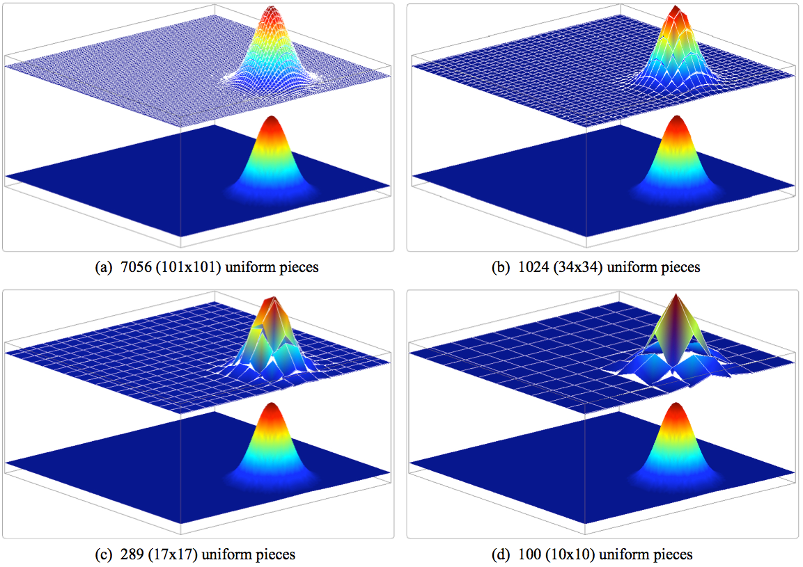
Figure 38.4: Four IvP functions approximating the same underlying function: Each IvP function uses a different number of uniform pieces.
| Case | Edge Size | Pieces | Layout | Worst Error | Avg Error | Time (ms) |
| 1 | 3 | 27889 | (167x167) | 0.0761 | 0.0014 | 656.4 |
| 2 | 5 | 1000 | (100x100) | 0.3019 | 0.0048 | 160.0 |
| 3 | 7 | 5184 | (72x72) | 0.6720 | 0.0104 | 83.3 |
| 4 | 10 | 2500 | (50x50) | 1.4589 | 0.0232 | 39.9 |
| 5 | 15 | 1156 | (34x34) | 3.4532 | 0.0551 | 18.9 |
| 6 | 20 | 625 | (25x25) | 5.5855 | 0.1014 | 10.4 |
| 7 | 25 | 400 | (20x20) | 7.79764 | 0.1585 | 6.5 |
| 8 | 30 | 289 | (17x17) | 12.0347 | 0.2303 | 4.7 |
| 9 | 40 | 169 | (13x13) | 24.2977 | 0.3919 | 2.8 |
| 10 | 50 | 100 | (10x10) | 18.2113 | 0.5917 | 1.6 |
| 11 | 75 | 49 | (7x7) | 42.0652 | 1.2143 | 0.9 |
| 12 | 100 | 25 | (5x5) | 30.3938 | 2.0285 | 0.5 |
Table 38.1: IvP function configurations and metrics: The relationship between piece size, accuracy and construction time is shown for varying uniform piece size. Four of the row entries are rendered in Figure 38.4.
38.4 The Full Reflector Interface Implementation [top]
The following functions define the interface to the Reflector tool. In constructing and setting parameters, the instance maintains a Boolean flag indicating if any fatal configuration errors were detected. In such cases, a warning string is generated for optional retrieval, and the error renders the instance effectively useless, never yielding an IvP function when requested. Example usage is provided in Listing 38.6.
- OF_Reflector(AOF*): The constructor takes a single argument, a pointer to the underlying function to be approximated by the Reflector. The AOF instance contains an instance of the IvPDomain which will also be the IvPDomain of any IvP functions created with the Reflector.
- int create(int pieces=-1): This function generates a new IvP function based on the prevailing parameter settings at the time of invocation. Many of the parameters affecting the form of the function are settable separately in the setParam() function, including the parameter specifying the number of pieces. If the optional pieces argument is provided in this function call, and if the value of the argument is
 , this overrides any piece count request set otherwise. This function will create an IvP function that the user can then obtain via the function extractIvPFunction() described below. The integer value returned is the number of pieces in the newly created IvP function. A value of zero indicates something has gone wrong.
- IvPFunction *extractIvPFunction(): This function returns a new IvP function built during a prior invocation of the create() function described above. If an error was encountered in either the parameter setting attempts, or in the invocation of the create() function, this function will simply return the NULL pointer. When the IvP function is extracted from the Reflector, an IvPFunction instance is created from the heap that needs to be later deleted. The Reflector tool does not delete this. It is the responsibility of the caller. Typically this tool is used within a behavior, and the behavior passes the IvP function to the helm and the helm deletes all IvP functions.
- string getWarnings(): When or if problems are encountered in setting the parameters, the Reflector appends a message to a local warning string. This string can be retrieved by this function.
- bool stateOK(): This function returns true if no errors were encountered during configuration attempts, otherwise it returns false. If an error has been encountered, this state cannot be reversed. The instance has been rendered effectively useless. To gain insight into the nature of the error, the getWarnings() function above can be consulted.
- bool setParam(string param, string value): This function is used for setting parameters on many optional tools more advanced than specifying the number of pieces to be used in a simple uniform function. An overview is provided here, with more detailed deferred to later sections that cover the advanced tools.
- uniform_amount: The amount of pieces to use in the creation of a simple uniform function. Alternatively can be supplied in the call to create() as described above.
- uniform_piece: A string description of the size and shape of a piece used during the creation of a pure uniform function. Details described in Section 39.1.2.
- strict_range: When set to true, the range of the linear interior function is guaranteed to stay within the range of any sampled points of the underlying function, even if a better overall fit could be obtained otherwise. The default is true.
- refine_region: A string description of a region of the IvP domain within which further directed refinement is requested. See Section 39.1.3.
- refine_piece: A string description of the size and shape of uniform pieces to be used within a region of directed refinement. See Section 39.3.
- refine_point: A string description of a point within the IvP domain to direct further refinement. See Section 39.3.
- smart_amount: The number of pieces to use in the smart refinement algorithm, beyond the number of pieces used in an initial simple uniform function. See Section 39.4.
- smart_percent: The number of pieces to use in the smart refinement algorithm specified as a percentage of the number of pieces used in an initial simple uniform function. See Section 39.4
- smart_thresh: A threshold given in terms of worst noted error between the IvP function and the underlying function, below which the smart refinement algorithm will cease further refinement. See Section 39.4.
- auto_peak: Set to either true or false indicating whether the auto-peak algorithm should be applied. See Section 39.5.
- auto_peak_max_pcs: The maximum amount of new pieces added to an IvP function during the auto-peak heuristic. See Section 39.5.
- bool setParam(string param, double value): The parameters that may be set via this function may also be set via the setParam() function above where the value parameter is a string. This alternate method is implemented solely as a convenience to the caller.
- uniform_amount: See above.
- smart_amount: See above.
- smart_percent: See above.
- smart_thresh: See above.
- auto_peak_max_pcs: See above.
Page built from LaTeX source using the texwiki program.