moos-ivp.org IvP ManPages Pavlab MIT 2.680 LAMSS Goby NOWISTHETIMEFORALLGOODMENTOCO NOWISTHETIMEFORALN Edit

6 IvP Helm Autonomy

6.1 Overview
     6.1.1 The Influence of Brooks, Stallman and Dantzig on the IvP Helm
     6.1.2 Traditional and Non-traditional Aspects of the IvP Behavior-Based Helm
     6.1.3 Two Layers of Building Autonomy in the IvP Helm
6.2 Inside the Helm - A Look at the Helm Iterate Loop
     6.2.1 Step 1 - Reading Mail and Populating the Info Buffer
     6.2.2 Step 2 - Evaluation of Mode Declarations
     6.2.3 Step 3 - Behavior Participation
     6.2.4 Step 4 - Behavior Reconciliation
     6.2.5 Step 5 - Publishing the Results to the MOOSDB
6.3 Mission Behavior Files
     6.3.1 Variable Initialization Syntax
     6.3.2 Behavior Configuration Syntax
     6.3.3 Hierarchical Mode Declaration Syntax
6.4 Hierarchical Mode Declarations
     6.4.1 Background
     6.4.2 Behavior Configuration Without Hierarchical Mode Declarations
     6.4.3 Syntax of Hierarchical Mode Declarations - The Bravo Mission
     6.4.4 A More Complex Example of Hierarchical Mode Declarations
     6.4.5 Monitoring the Mission Mode at Run Time
6.5 Behavior Participation in the IvP Helm
     6.5.1 Behavior Run Conditions
     6.5.2 Behavior Run Conditions and Mode Declarations
     6.5.3 Behavior Run States
     6.5.4 Behavior Flags and Behavior Messages
     6.5.5 Monitoring Behavior Run States and Messages During Mission Execution
6.6 Behavior Reconciliation in the IvP Helm - Multi-Objective Optimization
     6.6.1 IvP Functions
     6.6.2 The IvP Build Toolbox
     6.6.3 The IvP Solver and Behavior Priority Weights
     6.6.4 Monitoring the IvP Solver During Mission Execution

6.1 Overview [top]

An autonomous helm is primarily an engine for decision making. The IvP Helm uses a behavior-based architecture to organize its decision making and is distinctive in the manner in which it resolves competition between competing behaviors - it performs multi-objective optimization on their collective output using a mathematical programming model called interval programming. Here the IvP Helm architecture is described and the means for configuring it given a set of behaviors and a set of mission objectives.

6.1.1 The Influence of Brooks, Stallman and Dantzig on the IvP Helm [top]

The notion of a behavior-based architecture for implementing autonomy on a robot or unmanned vehicle is most often attributed to Rodney Brooks' Subsumption Architecture, [24]. A key principle at the heart of Brooks' architecture and arguably the primary reason its appeal has endured, is the notion that autonomy systems can be built incrementally. Notably, Brooks' original publication pre-dated the arrival of Open Source software and the Free Software Foundation founded by Richard Stallman. Open Source software is not a pre-requisite for building autonomy systems incrementally, but it has the capability of greatly accelerating that objective. The development of complex autonomy systems stands to significantly benefit if the set of developers at the table is large and diverse. Even more so if they can be from different organizations with perhaps even the loosest of overlap in interest regarding how to use the collective end product.

As discussed in Section 2.5, a key issue in behavior-based autonomy has been the issue of action selection, and the IvP Helm is distinct in this regard with the use of multi-objective optimization and interval programming. The algorithm behind interval programming, as well as the term itself, was motivated by the mathematical programming model, linear programming, developed by George Dantzig, [27]. The key idea in linear programming is the choice of the particular mathematical construct that comprises an instance of a linear programming problem - it has enough expressive flexibility to represent a huge class of practical problems, and the constructs can be effectively exploited by the simplex method to converge quickly even on very large problem instances. The constructs used in interval programming to represent behavior output (piecewise linear functions) were likewise chosen to have enough expressive behavior, and due to the opportunity to develop solution algorithms that exploit the piecewise linear constructs.

6.1.2 Traditional and Non-traditional Aspects of the IvP Behavior-Based Helm [top]

The IvP Helm indeed takes its motivation from early notions of the behavior-based architecture, but is also quite different in many regards. The notion of behavior independence to temper the growth of complexity in progressively larger systems is still a principle closely followed in the IvP Helm. Behaviors may certainly influence one another from one iteration to the next, as we'll see in discussions in this section. This was also evident in the Alpha example mission in Section 4 where the completion of the Survey behavior triggered the Return behavior. But within a single iteration, the output generated by a single behavior is not affected at all by what is generated by other behaviors in the same iteration. The only inter-behavior "communication" realized within an iteration comes when the IvP solver reconciles the output of multiple behaviors. The independence of behaviors not only helps a single developer manage the growth of complexity, but it also limits the dependency between developers. A behavior author need not worry that a change in the implementation of another behavior by another author requires subsequent recoding of one's own behavior(s).

Certain aspects of behaviors in the IvP Helm may also be a departure from some notions traditionally associated (fairly or not) with behavior-based architectures:

Behaviors have state. IvP behaviors are instances of a class with a fairly simple interface to the helm. Inside they may be arbitrarily complex, keep histories of observed sensor data, and may contain algorithms that could be considered "reactive" or "plan-based".
Behaviors influence each other between iterations. The primary output of behaviors is their objective function, ranking the utility of candidate actions. IvP behaviors may also generate variable-value posts to the MOOSDB observable by behaviors on the next helm iteration. In this way they can explicitly influence other behaviors by triggering or suppressing their activation or even affecting the parameter configuration of other behaviors.
Behaviors may accept externally generated plans. The input to a behavior can be anything represented by a MOOS variable, and perhaps generated by other MOOS processes outside the helm. It is allowable to have one or more planning engines running on the vehicle generating output consumed by one or more behaviors.
Several instances of the same behavior. Behaviors generally accept a set of configuration parameters that allow them to be configured for quite different tasks or roles in the same helm and mission. Different waypoint behaviors, for example, can be configured for different components of a transit mission. Or different collision avoidance behaviors can be instantiated for different contacts.
Behaviors can be run in a configurable sequence. Due to the condition and endflag parameters defined for all behaviors, a sequence of behaviors can be readily configured into a larger mission plan.
Behaviors rate actions over a coupled decision space. IvP functions generated by behaviors are defined over the Cartesian product of the set of vehicle decision variables. This is distinct from the de-coupled decision making style proposed in [17] and [19] - early advocates of multi-objective optimization in behavior-based action selection.

6.1.3 Two Layers of Building Autonomy in the IvP Helm [top]

The autonomy in play on a vehicle during a particular mission is the product of two distinct efforts - (1) the development of vehicle behaviors and their algorithms, and (2) mission planning via the configuration of behaviors and mode declarations. The former involves the writing of new source code, and the latter involves the editing of mission behavior files, such as the simple example for the Alpha example mission in Listing 4.1.

6.2 Inside the Helm - A Look at the Helm Iterate Loop [top]

Like other MOOS applications, the IvP Helm implements an Iterate() loop within which the basic function of the helm is executed. Components of the Iterate() loop, with respect to the behavior-based architecture, are described in this section. The basic flow, in five steps, is depicted in Figure 6.1. Description of the five components follow.

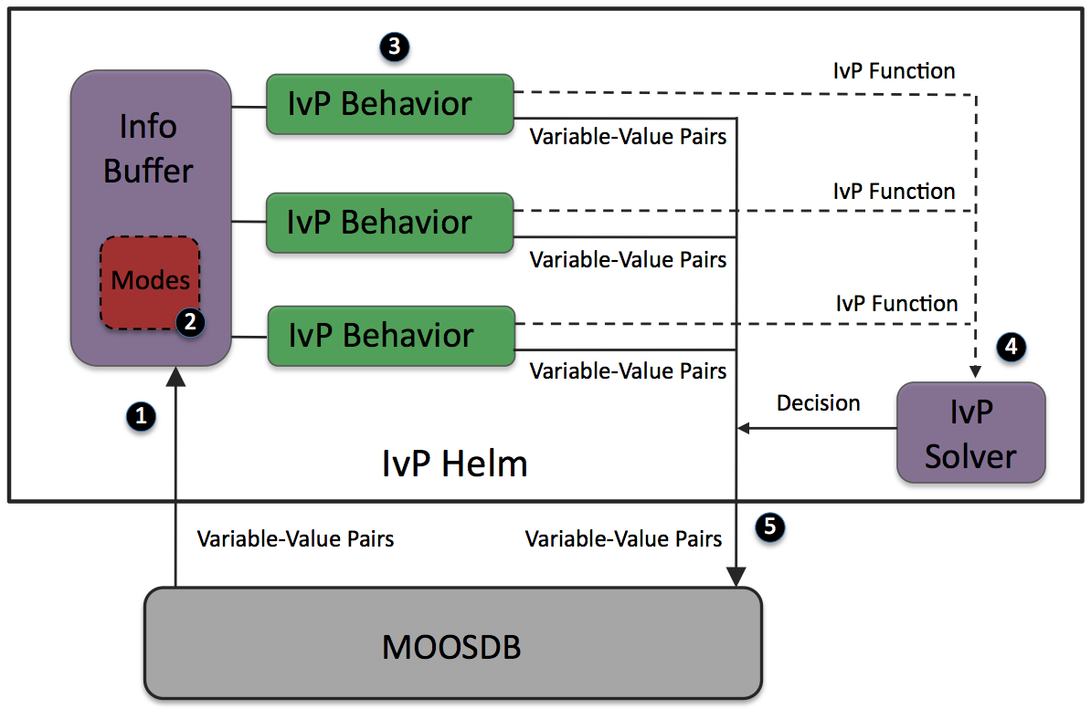
Figure 6.1: The pHelmIvP Iterate Loop: (1) Mail is read from the MOOSDB. It is parsed and stored in a local buffer to be available to the behaviors, (2) If there were any mode declarations in the mission behavior file they are evaluated at this step. (3) Each behavior is queried for its contribution and may produce an IvP function and a list of variable-value pairs to be posted to the MOOSDB at the end of the iteration, (4) the objective functions are resolved to produce an action, expressible as a set of variable-value pairs, (5) all variable-value pairs are published to the MOOSDB for other MOOS processes to consume.

6.2.1 Step 1 - Reading Mail and Populating the Info Buffer [top]

The first step of a helm iteration occurs outside the Iterate() loop. As depicted in Figure 3.1, a MOOS application will read its mail by executing its OnNewMail() function just prior to executing its Iterate() loop if there is any mail in its in-box. The helm parses mail to maintain its own information buffer which is also a mapping of variables to values. This is done primarily for simplicity - to ensure that each behavior is acting on the same world state as represented by the info buffer. Each behavior has a pointer to the buffer and is able to query the current value of any variable in the buffer, or get a list of variable-value changes since the previous iteration.

6.2.2 Step 2 - Evaluation of Mode Declarations [top]

Once the information buffer is updated with all incoming mail, the helm evaluates any mode declarations specified in the behavior file. Mode declarations are discussed in Section 6.4. In short, a mode is represented by a string variable that is reset on each iteration based on the evaluation of a set of logic expressions involving other variables in the buffer. The variable representing the mode declaration is then available to the behavior on the current iteration when it, for example, evaluates its condition parameters. A condition for behavior participating in the current iteration could therefore read something like condition = (MODE==SURVEYING). The exact value of the variable MODE is set during this step of the Iterate() loop.

6.2.3 Step 3 - Behavior Participation [top]

In the third step much of the work of the helm is realized by giving each behavior a chance to participate. Each behavior is queried sequentially - the helm contains no separate threads in this regard. The order in which behaviors is queried does not affect the output. This step contains two distinct parts for each behavior - (1) Determination of whether the behavior will participate, and (2) production of output if it is indeed participating on this iteration. Each behavior may produce two types of information as the Figure 6.1 indicates. The first is an objective function (or "utility" function) in the form of an IvP function. The second kind of behavior output is a list of variable-value pairs to be posted by the helm to the MOOSDB at the end of the Iterate() loop. A behavior may produce both kinds of information, neither, or one or the other, on any given iteration.

6.2.4 Step 4 - Behavior Reconciliation [top]

In the fourth step depicted in Figure 6.1, the IvP functions are collected by the IvP solver to produce a single decision over the helm's decision space. Each function is an IvP function - an objective function that maps each element of the helm's decision space to a utility value. In this case the functions are of a particular form - piecewise linearly defined. That is, each piece is an interval of the decision space with an associated linear function. Each function also has an associated weight and the solver performs multi-objective optimization over the weighted sum of functions (in effect a single objective optimization at that point). The output is a single optimal point in the decision space. For each decision variable the helm produces another variable-value pair, such as DESIRED_SPEED = 2.4 for publication to the MOOSDB.

6.2.5 Step 5 - Publishing the Results to the MOOSDB [top]

In the last step, the helm simply publishes all variable-value pairs to the MOOSDB, some of which were produced directly by the behaviors, and some of which were generated as output from the IvP Solver. The helm employs the duplication filter described in Section 5.8, only on the variable-value pairs generated directly from the behaviors, and not the variable-value pairs generated by the IvP solver that represent a decision in the helm's domain. For example, even if the decision about a vehicle's depth, represented by the variable DESIRED_DEPTH produced by the helm were unchanged for 5 minutes of operation, it would be published on each iteration of the helm. To do otherwise could give the impression to consumers of the variable that the variable is "stale", which could trigger an unwanted override of the helm out of concern for safety.

6.3 Mission Behavior Files [top]

The helm is configured for a particular mission primarily through one or more mission behavior files, typically with a *.bhv suffix. Behavior files have three types of entries, usually but not necessarily kept in three distinct parts - (1) variable initializations, (2) behavior configurations, and (3) hierarchical mode declarations. These three parts are discussed below. The example alpha.bhv file in Listing 4.1 did not contain hierarchical mode declarations, but does contain examples of variable initializations and behavior configurations.

6.3.1 Variable Initialization Syntax [top]

The syntax for variable initialization is fairly straight-forward:

    initialize  <variable> = <value>
    ...
    initialize  <variable> = <value>

Multiple initializations may be declared on a single line by separating each variable-value pair with a comma. The keyword initialize is case insensitive. The <variable> is indeed case sensitive since it will be published to the MOOSDB and MOOS variables are case sensitive when registered for by a client. The <value> may or may not be case sensitive depending on whether or not a client registering for the variable regards the case. Considering again the helm Iterate() loop depicted in Figure 6.1, variable initializations are applied to the helm's information buffer prior to the very first helm iteration, but are posted to the MOOSDB at the end of the first helm iteration.

By default, an initialization will overwrite any prior value posted to the MOOSDB. There may be situations, however, where the user's desired effect is that the initialization only be applied if no other value has yet been written to the given MOOS variable. The syntax in this case would be:

    initialize_  <variable> = <value>    // Deferring to prior posts if any

By using the "underscore" version of the initialize declaration, the helm will first register with the MOOSDB for the given variable, wait an iteration until it has had chance to receive mail from the MOOSDB on that variable, and only initialize the variable if nothing is otherwise known about that variable. (Note to the very discerning reader: Such an initialization also includes both an update to the helm's information buffer and a post to the MOOSDB. Posts to the MOOSDB by the helm, as part of a variable initialization, will indeed show up in the helm's incoming mailbox on the next iteration, but they are tagged in such a way as to be ignored by the helm. This is to ensure that they do not "collide" with posts made by other processes.)

6.3.2 Behavior Configuration Syntax [top]

The bulk of the helm configuration is done with individual behavior parameter blocks which have the following form:

  Behavior = <behavior-type>
  {
    <parameter> = <value>
    ...
    <parameter> = <value>
  }

The first line is a declaration of the behavior type. The keyword Behavior is not case sensitive, but the <behavior-type> is. This is followed by an open brace on a separate line. Each subsequent line sets a particular parameter of the behavior to a given value. The behavior configuration concludes with a close brace on a separate line. The issue of case sensitivity for the <parameter> and <value> entries is a matter determined by the individual behavior implementation.

As a convention (not enforced in any way) general behavior parameters, defined at the IvP Behavior superclass level, are grouped together and listed before parameters that apply to a specific behavior. For example, in the Alpha example in Listing 4.1, the general behavior parameters are listed on lines 8-12 and 22-25, but the parameters specific to the waypoint behavior, speed, radius, and points, follow in a separate block. Generally it is not mandatory to provide a parameter-value pair for each parameter defined for a behavior, given that meaningful defaults are in place within the behavior implementation. Some parameters are indeed mandatory however. Documentation for the individual behavior should be consulted. Multiple instances of a behavior type are allowed, as in the Alpha example where there are two waypoint behaviors - one for traversing a set of points, and one for returning to a vehicle recovery point. Each behavior should have its own unique value provided in the name parameter.

6.3.3 Hierarchical Mode Declaration Syntax [top]

Hierarchical Mode Declarations are covered in depth in Section 6.4, but the syntax is briefly discussed here. A behavior file contains a set of declaration blocks of the form:

  Set <mode-variable-name> = <mode-value>
  {
    <mode-variable-name> = <parent-value>
    <condition>
    . . .
    <condition>
  } <else-value>

A tree will be formed where each node in the tree is described from the above type of declaration. The keyword Set is case insensitive. The <mode-variable-name>, <parent-value> and <else-value> are case sensitive. The <condition> entries are treated exactly as with the condition parameter for behaviors, see Section 6.5.1.

As indicated in Figure 6.1, the value of each mode variable is reset at the outset of the Iterate() loop, after the information buffer is updated with incoming mail. A mode variable is set by progressing through each declaration block, and determining whether the conditions are met. Thus the ordering of the declaration blocks is significant - the specification of parent should be made prior to that of a child. Examples are further discussion can be found below in Section 6.4.

6.4 Hierarchical Mode Declarations [top]

Hierarchical mode declarations (HMDs) are an optional feature of the IvP Helm for organizing the behavior activations according to declared mission modes. Modes and sub-modes can be declared, in line with a mission planner's own concept of mission evolution, and behaviors can be associated with the declared modes. In more complex missions, it can facilitate mission planning (in terms of less time and better detection of human errors), and it can facilitate the understanding of exactly what is happening in the helm - during the mission execution and in post-analysis.

6.4.1 Background [top]

A trend of unmanned vehicle usage can be characterized as being increasingly less of the shorter, scripted variety to be increasingly more of the longer, adaptive mission variety. A typical mission in our own lab five years ago would contain a certain set of tasks, typically waypoints and ultimately a rendezvous point for recovering the vehicle. Data acquired during deployment was off-loaded and analyzed later in the laboratory. What has changed? The simultaneous maturation of acoustic communications, on-board sensor processing, and longer vehicle battery life has dramatically changed the nature of mission configurations. The vehicle is expected to adapt to both the phenomena it senses and processes on board, as well as adapt its operation given field-control commands received via acoustic, radio or satellite communications. Multi-vehicle collaborative missions are also increasingly viable due to lower vehicle costs and mature acomms capabilities. In such cases a vehicle is not only adapting to sensed phenomena and field commands, but also to information from collaborating vehicles.

Our missions have evolved from having a finite set of fixed tasks to be composed instead of a set of modes, an initial mode when launched, an understanding of what brings us from one mode to another, and what behaviors are in play in each mode. Modes may be entered and exited any number of times, in exact sequences unknown at launch time, depending on what they sense and how they are commanded in the field.

6.4.2 Behavior Configuration Without Hierarchical Mode Declarations [top]

Behaviors can be configured for a mission without the use of hierarchical mode declarations - support for HMDs is a relatively recent addition to the helm. HMDs are a tool for organizing which behaviors are idle or participating in which circumstances. Consider the alpha example mission in Section 4, and the behavior file in Listing 4.1. By examination of the behavior file, and experimenting a bit with the viewer during simulation, the vehicle apparently is always in one of three modes - (a) idle, (b) surveying the waypoints, or (c) returning to the launch point. This is achieved by the condition parameters for the two behaviors. There are only two variables involved in the behavior conditions, DEPLOY and RETURN. If restricted to Boolean values, the below table confirms the observation that there are only three possible modes.

DEPLOY	RETURN	Mode
true	true	Returning
true	false	Surveying
false	true	Idle
false	false	Idle

Table 6.1: Possible modes implied by the condition parameters in the alpha mission in Listing 4.1.

There are a couple drawbacks with this however. First, the modes are to be inferred from the behavior conditions and this is not trivial in missions with larger behavior files. Mapping the behavior conditions to a mode is useful both in mission planning and mission monitoring. In the alpha mission, in order to understand at any given moment what mode the vehicle is in, the two variables need to be monitored, and the above table internalized. The second drawback is the increased likelihood of error, in the form of unintentionally being in two modes at the same time, or being in an undefined mode. For example, line 11 in Listing 4.1 really should read RETURN != true, and not RETURN = false. Since there is no Boolean type for MOOS variables, this variable could be set to "False" and the condition as it reads on line 11 in Listing 4.1 would not be satisfied, and the vehicle would be in the idle state, despite the fact that DEPLOY may be set to true. These problems are alleviated by the use of hierarchical mode declarations.

6.4.3 Syntax of Hierarchical Mode Declarations - The Bravo Mission [top]

An example is provided showing of the use of hierarchical mode declarations by extending the Alpha mission described in Section 4. This example mission is dubbed the "Bravo" mission in the directory s2_bravo alongside the Alpha mission s1_alpha in the MOOS-IvP distribution (Section 4.1). It is also given fully in Listing 6.1 on the next page. The implicit modes of the Alpha mission, described in Table 6.1, are explicitly declared in the Bravo behavior file to form the following hierarchy:

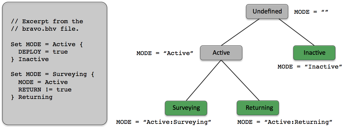
Figure 6.2: Hierarchical modes for the Bravo mission: The vehicle will always be in one of the modes represented by a leaf node. A behavior may be associated with any node in the tree. If a behavior is associated with an internal node, it is also associated with all its children.

The hierarchy in Figure 6.2 is formed by the mode declaration constructs on the left-hand side, taken as an excerpt from the bravo.bhv file. After the mode declarations are read when the helm is initially launched, the hierarchy remains static thereafter. The hierarchy is associated with a particular MOOS variable, in this case the variable MODE. Although the hierarchy remains static, the mode is re-evaluated at the outset of each helm iteration based on the conditions associated with nodes in the hierarchy. The mode evaluation is represented as a string in the variable MODE. As shown in Figure 6.2 the variable is the concatenation of the names of all the nodes. The mode evaluation begins sequentially through each of the blocks. At the outset the value of the variable MODE is reset to the empty string. After the first block in Figure 6.2 MODE will be set to either "Active" or "Inactive". When the second block is evaluated, the condition "MODE=Active" is evaluate based on how MODE was set in the first block. For this reason, mode declarations of children need to be listed after the declarations of parents in the behavior file.

Once the mode is evaluated, at the outset of the helm iteration, it is available for use in the conditions of the behaviors, as in lines 20 and 23 in Listing 6.1. Note the "==" relation in lines 18 and 36. This is a string-matching relation that matches when one side matches exactly one of the components in the other side's colon-separated list of strings. Thus "Active" == "Active:Returning", and "Returning" == "Active:Returning". This is to allow a behavior to be easily associated with an internal node regardless of its children. For example if a collision-avoidance behavior were to be added to this mission, it could be associated with the "Active" mode rather than explicitly naming all the sub-modes of the "Active" mode.

Listing 6.1 - The Bravo Mission - Use of Hierarchical Mode Declarations.

   1  initialize   DEPLOY = false
   2  initialize   RETURN = false
   3     
   4  //------------------- Declaration of Hierarchical Modes
   5  set MODE = ACTIVE {
   6    DEPLOY = true
   7  } INACTIVE
   8   
   9  set MODE = SURVEYING {
  10    MODE = ACTIVE
  11    RETURN != true
  12  } RETURNING
  13   
  14  //----------------------------------------------
  15  Behavior = BHV_Waypoint
  16  { 
  17    name      = waypt_survey
  18    pwt       = 100
  19    condition = MODE == SURVEYING
  20    endflag   = RETURN = true
  21    perpetual = true
  22  
  23            lead = 8
  24     lead_damper = 1
  25           speed = 2.0   // meters per second
  26          radius = 4.0
  27       nm_radius = 10.0
  28          points = 60,-40:60,-160:150,-160:180,-100:150,-40
  29          repeat = 1
  30  }
  31    
  32  //----------------------------------------------
  33  Behavior = BHV_Waypoint
  34  {
  35    name       = waypt_return
  36    pwt        = 100
  37    condition  = MODE == RETURNING
  38    perpetual  = true
  39    endflag    = RETURN = false
  40    endflag    = DEPLOY = false
  41  
  42         speed = 2.0
  43        radius = 2.0
  44     nm_radius = 8.0
  45         point = 0,0
  46  }

6.4.4 A More Complex Example of Hierarchical Mode Declarations [top]

The Bravo example given above, while having the benefit of being a working example distributed with the codebase, is not complex. In this section a modestly complex, although fictional, hierarchy is provided to highlight some issues with the syntax. The hierarchy with the corresponding mode declarations are shown in Figure 6.3. The declarations are given in the order of layers of the tree ensuring that parents are declared prior to children. As with the Bravo example in Figure 6.2, the nodes that represent realizable modes are depicted in the darker (green) color.

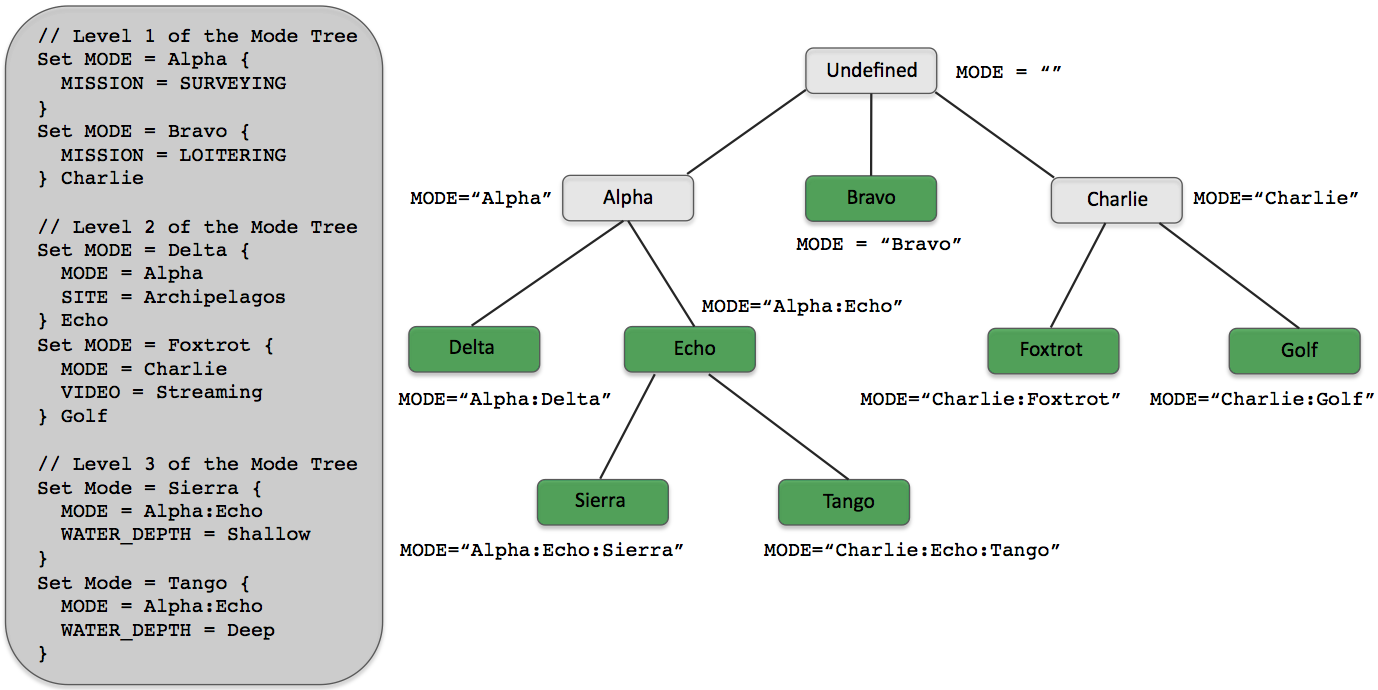
Figure 6.3: Example Hierarchical Mode Declaration: The hierarchy on the right is constructed from the set of mode declarations on the the left (with fictional conditions). Darker nodes represent modes that are realizable through some combination of conditions.

The "Alpha" mode for example is not realizable since it has the children "Delta" and "Echo", with the latter being set as the <else-value> if the conditions of the former at not met. The "Bravo" mode is realizable since it has no children. The "Echo" mode is realizable despite having children because the "Tango" mode is not the <else-value> of the "Sierra" mode declaration. For example, if the following three conditions hold, (a) "MISSION=SURVEYING", (b) "SITE!=Archipelagos", and (c) "WATER_DEPTH=Medium", then the value of the variable MODE would be set to "Alpha:Echo". Finally, note that the condition in the "Sierra" declaration, "MODE=Alpha:Echo", is specified fully, i.e., "MODE=Echo" would not achieve the desired result.

6.4.5 Monitoring the Mission Mode at Run Time [top]

The mission mode can be monitored at run time in a couple ways. First, since the mode variable is posted as a MOOS variable, any MOOS scope tool will work, e.g., uXMS, uMS, uHelmScope. Using uHelmScope, the mission variable can be monitored as part of the basic MOOSDB scoping capability, but it is also displayed as part of the uHelmScope app, and in the AppCasting output of pHelmIvP.

The uHelmScope tool also has a mode in which the entire mode hierarchy may be rendered - solely to provide a visual confirmation that the hierarchy specified with the mode declarations in the behavior file does in fact correspond to what the user intended. Currently there are no tools to automatically render the mode hierarchy in a manner like the right hand side of Figure 6.3. The uHelmScope output for the example in Figure 6.3 is shown in listing 6.2 below.

Listing 6.2 - The mode hierarchy output from uHelmScope for the example in Figure 6.3.

   1   ModeSet Hierarchy: 
   2   ---------------------------------------------- 
   3   Alpha
   4       Delta
   5       Echo
   6           Sierra
   7           Tango
   8   Bravo
   9   Charlie
  10       Foxtrot
  11       Golf
  12   ---------------------------------------------- 
  13   CURENT MODE(S): Charlie:Foxtrot
  14                                                               
  15   Hit 'r' to resume outputs, or SPACEBAR for a single update

More on this feature of the uHelmScope can be found in the uHelmScope documention, [29]. It's worth noting that poking the value of a mode variable will have no effect on the helm operation. The mission mode cannot be commanded directly. The mode variable is reset at the outset of the helm iteration, and the helm doesn't even register for mail on mode variables.

6.5 Behavior Participation in the IvP Helm [top]

The primary work of the helm comes when the behaviors participate and do their thing, at each round of the helm Iterate() loop. As depicted in Figure 6.1, once the mode has been re-evaluated taking into consideration newly received mail, it is time for the behaviors (well, some at least) to step up and do their thing.

6.5.1 Behavior Run Conditions [top]

On any single iteration a behavior may participate by generating an objective function to influence the helm's output over its decision space. Not all behaviors participate in this regard, and the primary criteria for participation is whether or not it has met each of its "run conditions". These are the conditions laid out in the behavior file of the form:

    condition = <logic-expression>

The <logic-expression> syntax is described in Appendix 43. Conditions are built from simple relational expressions, the comparison of MOOS variables to specified literal values, or the comparison of MOOS variables to one another. Conditions may also involve Boolean logic combinations of relation expressions. A behavior may base its conditions on any MOOS variable such as:

    condition = (DEPLOY=true) and (STATION_KEEP != true)

A run condition may also be expressed in terms of a helm mode, as described in the next Section 6.5.2 such as:

    condition = (MODE == LOITERING)

All MOOS variables involved in run condition expressions are automatically subscribed for by the helm to the MOOSDB.

6.5.2 Behavior Run Conditions and Mode Declarations [top]

The use of hierarchical mode declarations potentially simplify the expressions used as run conditions. The conditions in practice could be limited to:

    condition = <mode-variable> = <mode-value>, or
    condition = <mode-variable> == <mode-value>.

Conditions were used in this way with the Bravo mission in Listing 6.1, as an alternative to their usage in the Alpha mission example in Listing 4.1.

Note the use of the double-equals relation above. This relation is used for matching against the strings used to represent the hierarchical mode. The two strings match if the ordered components of one side are a subset of the ordered components of the other. Components are colon-separated. For example, using the illustrative hierarchy from Figure 6.3:

        "Alpha:Echo:Sierra" == "Sierra"
        "Alpha:Echo:Sierra" == "Echo:Sierra"
        "Alpha:Echo:Sierra" == "Alpha"
                   "Sierra" == "Alpha:Echo:Sierra"
          "Charlie:Foxtrot" == "Charlie:Foxtrot"

        "Alpha:Echo:Sierra" != "Alpha:Sierra"

6.5.3 Behavior Run States [top]

On any given helm iteration a behavior may be in one of four states depicted in Figure 6.4:

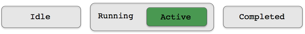
Figure 6.4: Behavior States: A behavior may be in one of these four states at any given iteration of helm Iterate() loop. The state is determined by examination of MOOS variables stored locally in the helm's information buffer.

Idle: A behavior is idle if it is not complete and it has not met its run conditions as described above in Section 6.5.1. The helm will invoke an idle behavior's onIdleState() function.
Running: A behavior is running if it has met its run conditions and it is not complete. The helm will invoke a running behavior's onRunState() function thereby giving the behavior an opportunity to contribute an objective function.
Active: A behavior is active if it is running and it did indeed produce an objective function when prompted. There are a number of reasons why a running behavior may not be active. For example, a collision avoidance behavior where the object of the behavior is sufficiently far away.
Complete: A behavior is complete when the behavior itself determines it to be complete. It is up to the behavior author to implement this, and some behaviors may never complete. The function setComplete() is defined generally at the behavior superclass level, for calling by a behavior author. This provides some some standard steps to be taken upon completion, such as posting of endflags, described below in Section 6.5.4. Once a behavior is in the complete state, it remains in that state permanently. All behaviors have a duration parameter defined to allow it to be configured to time-out if desired. When a time-out occurs the behavior state will be set to complete.

6.5.4 Behavior Flags and Behavior Messages [top]

Behaviors may post some number of messages, i.e., variable-value pairs, on any given iteration (see Figure 6.1). These message can be critical for coordinating behaviors with each other and to other MOOS processes. The can also be invaluable for monitoring and debugging behaviors configured for particular missions. To be more accurate, behaviors don't post messages to the MOOSDB, they request the helm to post messages on its behalf. The helm collects these requests and publishes them to the MOOSDB at the end of the Iterate() loop. It also filters them for successive duplicates as discussed in Section 5.8.

There is a standard method, configurable in the behavior file, for posting messages based on the run state of the behavior. These are referred to as behavior flags, and there are several types, endflag, idleflag, runflag, activeflag, inactiveflag, and spawnflag. The variable-value pairs representing each flag are set in the behavior file for the corresponding behavior. See line 11 in Listing 4.1 for example.

endflag: An endflag is posted once when or if the behavior enters the complete state. The variable-value pair representing the endflag is given in the endflag parameter in the behavior file. Multiple endflags may be configured for a behavior.
idleflag: An idleflag is posted by the helm when the behavior enters the idle state. The variable-value pair representing the idleflag is given in the idleflag parameter in the behavior file. Multiple idleflags may be configured for a behavior.
runflag: A runflag is posted by the helm when the behavior enters the running state from the idle state. A runflag is posted exactly when an idleflag is not. The variable-value pair representing the runflag is given in the runflag parameter in the behavior file. Multiple runflags may be configured for a behavior.
activeflag: An activeflag is posted by the helm when the behavior enters the active state. The variable-value pair representing the activeflag is given in the activeflag parameter in the behavior file. Multiple activeflags may be configured for a behavior.
inactiveflag: An inactiveflag is posted by the helm when the behavior enters a state that is not the active state. The variable-value pair representing the inactiveflag is given in the inactiveflag parameter in the behavior file. Multiple inactiveflags may be configured for a behavior.
spawnflag: An spawnflag is posted by the helm when templated behavior is spawned. Examples include the collision and obstacle avoidance behaviors. The variable-value pair representing the spawnflag is given in the spawnflag parameter in the behavior file. Multiple spawnflags may be configured for a behavior.

A runflag is meant to "complement" an idleflag, by posting exactly when the other one does not. Similarly with the inactiveflag and activeflag. The situation is shown in Figure 6.5:

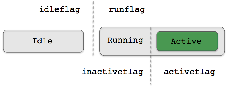
Figure 6.5: Behavior Flags: The four behavior flags idleflag, runflag, activeflag, and inactiveflag are posted depending on the behavior state and can be considered complementary in the manner indicated.

Behavior authors may implement their behaviors to post other messages as they see fit. For example the waypoint behavior used in the Alpha example in Section 4 also published the variable WPT_STAT with a status message similar to "vname=alpha,index=0,dist=124,eta=62" indicating the name of the vehicle, the index of the next point in the list of waypoints, the distance to that waypoint, and the estimated time of arrival, in seconds. (You might want to re-run the Alpha mission with uXMS scoping on this variable to watch it change as the mission unfolds.)

6.5.5 Monitoring Behavior Run States and Messages During Mission Execution [top]

each iteration by the helm into a single string and published in the variable IVPHELM_SUMMARY. This variable is subscribed for by the uHelmScope tool and behavior states are parsed from this variable and summarized in the main output of uHelmScope, as in the below excerpt:

  12  Behaviors Active: ---------- (1)
  13    waypt_survey (13.0) (pwt=100.00) (pcs=1227) (cpu=0.01) (upd=0/0)
  14  Behaviors Running: --------- (0)
  15  Behaviors Idle: ------------ (1)
  16    waypt_return (22.8)
  17  Behaviors Completed: ------- (0)

Behaviors are grouped into the four possible states, with a summary line for each state, e.g., lines 12, 14, 15, 17, containing the number of behaviors in that state in parentheses at the end of the line. Each behavior configured for the helm shows up on a dedicated line in the appropriate group, e.g., lines 13 and 16. In these lines immediately following the behavior name, the number of seconds is displayed in parentheses indicating how long the behavior has been in that state.

6.6 Behavior Reconciliation in the IvP Helm - Multi-Objective Optimization [top]

6.6.1 IvP Functions [top]

IvP functions are produced by behaviors to influence the decision produced by the helm on the current iteration (see Figure 6.1). The decision is typically comprised of the desired heading, speed, and depth but the helm decision space could be comprised of any arbitrary configuration (see Section 5.4.6). Some points about IvP functions:

IvP functions are piecewise linearly defined. Each piece is defined by an interval over some subset of the decision space, and there is a linear function associated with each piece (see Figure 6.7).
IvP functions are an approximation of an underlying function. The linear function for a single piece is the best linear approximation of the underlying function for the portion of the domain covered by that piece.
IvP domains are discrete with an upper and lower bound for each variable, so an IvP function may achieve zero-error in approximating an underlying function by associating a piece with each point in the domain. Behaviors seldom need to do so in practice however.
The Ivp function construct and IvP solver are generalizable to N dimensions.
The pieces in IvP functions need not be uniform size or shape. More pieces can be dedicated to parts of the domain that are harder to approximate with linear functions.
IvP functions need only be defined over a subset of the domain. Behaviors are not affected if the helm is configured for additional variables that a behavior may not care about. Behaviors that produce functions solely over vehicle depth are perfectly ok.

How are IvP functions built? The IvP Build Toolbox is a set of tools for creating IvP functions based on any underlying function defined over an IvP Domain. Many, if not all of the behaviors in this document make use of this toolbox, and authors of new behaviors have this at their disposal. A primary component of writing a new behavior is the development of the "underlying function", the function approximated by an IvP function with the help of the toolbox. The underlying function represents the relationship between a candidate helm decision and the expected utility with respect to the behavior's objectives. The IvP Toolbox is not covered in detail in this document, but an overview is given below.

6.6.2 The IvP Build Toolbox [top]

The IvP Toolbox is a set of tools (a C++ library) for building IvP functions. It is typically utilized by behavior authors in a sequence of library calls within a behavior's (C++) implementation. There are two sets of tools - the Reflector tools for building IvP functions in N dimensions, and the ZAIC tools for building IvP functions in one dimension as a special case. The Reflector tools work by making available a function to be approximated by an IvP function. The tools simply need this function for sampling. Consider the Gaussian function rendered below in Figure 6.6:

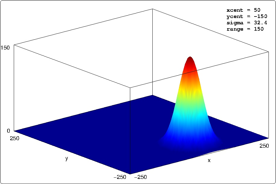
Figure 6.6: A rendering of the function 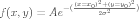where A = {\tt range} = 150, = {\tt sigma} = 32.4, = {\tt xcent} = 50, = {\tt ycent} = -150. The domain here for x and y ranges from -250 to 250.

The 'x' and 'y' variables, each with a range of [-250, 250], are discrete, taking on integer values. The domain therefore contains points, or possible decisions. The IvP Build Toolbox can generate an IvP function approximating this function over this domain by using a uniform piece size, as rendered in Figure 6.7. The only difference in these four piecewise function is the number and size of the piece. More pieces (Figure 6.7 (a)) results in a more accurate approximation of the underlying function, but takes longer to generate and creates further work for the IvP solver when the functions are combined. IvP functions need not use uniformly sized pieces.

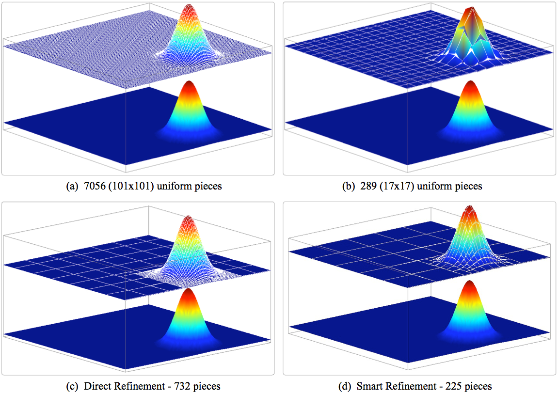
Figure 6.7: A rendering of four different IvP functions approximating the same underlying function: The function in (a) uses a uniform distribution of 7056 pieces. The function in (b) uses a uniform distribution of 1024 pieces. The function in (c) was created by first building a uniform distribution of 49 pieces and then focusing the refinement on a sub-domain of the function. This is called directed-refinement in the IvP Build toolbox. The function in (d) was created by first building a uniform function of 25 pieces and repeatedly refining the function based on which pieces were noted to have a poor fit to the underlying function. This is termed smart-refinement in the IvP Build toolbox.

By using the directed refinement option in the IvP Build Toolbox, an initially uniform IvP function can be further refined with more pieces over a sub-domain directed by the caller, with smaller uniform pieces of the caller's choosing. This is described more fully in the documentation for the IvP Build Toolbox. Using this tool requires the caller to have some idea where, in the sub-domain, further refinement is needed or desired. Often a behavior author indeed has this insight. For example, if one of the domain variables is vehicle heading, it may be good to have a fine refinement in the neighborhood of heading values close to the vehicle's current heading.

In other situations, insight into where further refinement is needed may not be available to the caller. In these cases, using the smart refinement option of the IvP Build Toolbox, an initially uniform IvP function may be further refined by asking the toolbox to automatically "grade" the pieces as they are being created. The grading is in terms of how accurate the linear fit is between the piece's linear function and the underlying function over the sub-domain for that piece. A priority queue is maintained based on the grades, and pieces where poor fits are noted, are automatically refined further, up to a maximum piece limit chosen by the caller. This is described more fully in the documentation for the IvP Build Toolbox

The Reflector tools work similarly in N dimensions and on multi-modal functions. The only requirement for using the Reflector tool is to provide it with access to the underlying function. Since the tool repetitively samples this function, a central challenge to the user of the toolbox is to develop a fast implementation of the function. In terms of the time consumed in generating IvP functions with the Reflector tool, the sampling of the underlying function is typically the long pole in the tent.

6.6.3 The IvP Solver and Behavior Priority Weights [top]

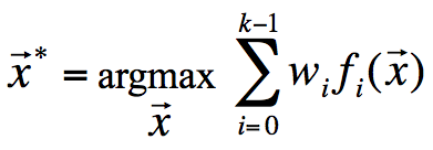
The IvP Solver collects a set of weighted IvP functions produced by each of the behaviors and finds a point in the decision space that optimizes the weighted combination. If each IvP objective function is represented by , and the weight of each function is given by , the solution to a problem with k functions is given by:

The algorithm is described in detail in [7], but is summarized in the following few points.

The search tree: The structure of the search algorithm is branch-and-bound. The search tree is comprised of an IvP function at each layer, and the nodes at each layer are comprised of the individual pieces from the function at that layer. A leaf node represents a single piece from each function. A node in the tree is realizable if the piece from that node and its ancestors intersect, i.e., share common points in the decision space.
Global optimality: Each point in the decision space is in exactly one piece in each IvP function and is thus in exactly one leaf node of the search tree. If the search tree is expanded fully, or pruned properly (only when the pruned out sub-tree does not contain the optimal solution), then the search is guaranteed to produce the globally optimal solution. The search algorithm employed by the IvP solver does indeed start with a fully expanded tree, and utilizes proper pruning to guarantee global optimality. The algorithm does allow for a parameter for guaranteed limited back-off from the global optimality - a quicker solution with a guarantee of being within a fixed percent of global optima. This option is not exposed to the IvP Helm which always finds the global optimum.
Initial solution: A key factor of an effective branch-and-bound algorithm is seeding the search with a decent initial solution. In the IvP Helm, the initial solution used is the solution (typically heading, speed, depth) generated on the previous helm iteration. Upon casual observation this appears to provide a speed-up by about a factor of two.

In cases where there is a "tie" between optimal decisions, the solution generated by the solver is non-deterministic. This is mitigated somewhat by the fact that the solution is seeded with the output of the previous iteration as discussed above.

6.6.4 Monitoring the IvP Solver During Mission Execution [top]

The performance of the solver can be monitored with the uHelmScope tool. The output shown below is an excerpt from an example mission. On line 5, the total time needed to solve the multi-objective optimization problem is given in seconds, and the max time need for all recorded loops is given in parentheses. It is zero here since there is only one objective function in this example. On line 6 is the total time for creating the IvP functions in all behaviors, with the max across all iterations in parentheses. On line 7 is the total loop time - the sum of the previous two lines. Active behaviors display useful information regarding the IvP solver. For example, on line 13, the Survey waypoint behavior had a priority weight of 100 and generated 1,227 pieces, taking 0.01 seconds of CPU time to create.

Listing 6.3 - Example uHelmScope output containing information about the IvP solver.

   1  ==============   uHelmScope Report  ============== DRIVE  (17)
   2    Helm Iteration: 66      (hz=0.38)(5)  (hz=0.35)(66)  (hz=0.56)(max)
   3    IvP functions:  1
   4    Mode(s):        Surveying
   5    SolveTime:      0.00    (max=0.00)
   6    CreateTime:     0.02    (max=0.02)
   7    LoopTime:       0.02    (max=0.02)
   8    Halted:         false   (0 warnings)
   9  Helm Decision: [speed,0,4,21] [course,0,359,360]
  10    speed = 3.00
  11    course = 177.00
  12  Behaviors Active: ---------- (1)
  13    waypt_survey (13.0) (pwt=100.00) (pcs=1227) (cpu=0.01) (upd=0/0)
  14  Behaviors Running: --------- (0)
  15  Behaviors Idle: ------------ (1)
  16    waypt_return (22.8)
  17  Behaviors Completed: ------- (0)
  18

The solver can be additionally monitored and analyzed through the two MOOS variables LOOP_CPU and CREATE_CPU published on each helm iteration. The former indicates the system wall time for building each IvP function and solving the multi-objective optimization problem, and the latter indicates just the time to create the IvP functions.

Page built from LaTeX source using the texwiki program.